Introduction
There are many techniques one can use to write information from a running Microsoft Office program. You can save data in a workbook, but this is unwieldy for saving small items, such as program settings. You can use ini files or the registry, but both can get complicated. Using the registry is more invasive than you may want to be, and it’s very hard to transfer registry settings among computers. One of the easiest methods to save and retrieve data is by using simple IO commands with text files. Such files are small, they are processed rapidly, they can be read with a simple text editor, and they can be easily copied from computer to computer.
Visual Basic I/O
Visual Basic contains some commands which are useful for fast and simple text file input and output. Since the Visual Basic for Applications (VBA) used to program Microsoft Office is based on VB, Excel and the other Office applications can use these commands to read and write text files. I frequently use this technique to save application settings or to store debugging information.
The VBA help files contain detailed information about the various IO commands. Rather than beat the topic to death, I’ll present a couple simple examples that write and read text from a text file, then I’ll show some practical examples. The reader is directed to the help files for further details.
The subroutine TextIODemoWrite, shown below, opens a specified text file, puts a simple text string into the file, then closes the file. Files are opened using integers starting with 1; the FreeFile function assigns the next available integer to the file, to prevent accidentally assigning the same integer to two files. When you Open the file, a buffer is allocated to it, and the access mode (e.g., Output) is assigned. If the file does not already exist, it is automatically created. Subsequent commands (Write and Close) refer to the file using its integer. Text can be written using Write or Print; refer to the help files for specifics. Closing a file deallocates the buffer and disassociates the file from the file number.
Sub TextIODemoWrite()
  Dim sFile As String
  Dim sText As String
  Dim iFileNum As Integer

  sFile = "C:\test\textio.txt"
  sText = "Testing 1 2 3."

  iFileNum = FreeFile
  Open sFile For Output As iFileNum
  Write #iFileNum, sText
  Close #iFileNum
End Sub
The subroutine TextIODemoRead below shows the reverse operation, opening a text file, retrieving some text, closing the text file, then displaying the text in a message box.
Sub TextIODemoRead()
  Dim sFile As String
  Dim sText As String
  Dim iFileNum As Integer

  sFile = "C:\test\textio.txt"

  iFileNum = FreeFile
  Open sFile For Input As iFileNum
  Input #iFileNum, sText
  Close #iFileNum
  MsgBox sText
End Sub
Save and Retrieve Settings
The VBA procedures above can be expanded to allow us to save settings for later retrieval. The simplistic approach used in function SaveSetting reads variable names and values from a file, and writes them to a temporary file. If the named variable already exists, its new value is written to the temporary file in place of the existing value. When all variables have been read and written, the original file is replaced by the new file.
SaveSetting uses some additional functions, IsFullName, FullNameToPath, FullNameToFileName, and FileExists, which are shown at the end of this article.
Function SaveSetting(sFileName As String, sName As String, _
      Optional sValue As String) As Boolean

  Dim iFileNumA As Long
  Dim iFileNumB As Long
  Dim sFile As String
  Dim sXFile As String
  Dim sVarName As String
  Dim sVarValue As String
  Dim lErrLast As Long

  ' assume false unless variable is successfully saved
  SaveSetting = False

  ' add this workbook's path if not specified
  If Not IsFullName(sFileName) Then
    sFile = ThisWorkbook.Path & "\" & sFileName
    sXFile = ThisWorkbook.Path & "\X" & sFileName
  Else
    sFile = sFileName
    sXFile = FullNameToPath(sFileName) & "\X" & FullNameToFileName(sFileName)
  End If

  ' open text file to read settings
  If FileExists(sFile) Then
    'replace existing settings file
    iFileNumA = FreeFile
    Open sFile For Input As iFileNumA
    iFileNumB = FreeFile
    Open sXFile For Output As iFileNumB
      Do While Not EOF(iFileNumA)
        Input #iFileNumA, sVarName, sVarValue
        If sVarName <> sName Then
          Write #iFileNumB, sVarName, sVarValue
        End If
      Loop
      Write #iFileNumB, sName, sValue
      SaveSetting = True
    Close #iFileNumA
    Close #iFileNumB
    FileCopy sXFile, sFile
    Kill sXFile
  Else
    ' make new file
    iFileNumB = FreeFile
    Open sFile For Output As iFileNumB
      Write #iFileNumB, sName, sValue
      SaveSetting = True
    Close #iFileNumB
  End If

End Function
The function is called using this syntax (bTest is declared as a Boolean). The filename (with or without path), the variable name, and the value are all passed to the function as strings. If a path is not included as part of the file name, then the workbook’s own path is used. The value of the function is true unless an error is encountered.
bTest = SaveSetting("C:\test\settings.txt", "test variable", "test value")Subroutine GetSetting enumerates the variables in the file until the named variable is found, then it extracts the value of this variable.
Function GetSetting(sFile As String, sName As String, _
      Optional sValue As String) As Boolean

  Dim iFileNum As Long
  Dim sVarName As String
  Dim sVarValue As String
  Dim lErrLast As Long

  ' assume false unless variable is found
  GetSetting = False

  ' add this workbook's path if not specified
  If Not IsFullName(sFile) Then
    sFile = ThisWorkbook.Path & "\" & sFile
  End If

  ' open text file to read settings
  If FileExists(sFile) Then
    iFileNum = FreeFile
    Open sFile For Input As iFileNum
      Do While Not EOF(iFileNum)
        Input #iFileNum, sVarName, sVarValue
        If sVarName = sName Then
          sValue = sVarValue
          GetSetting = True
          Exit Do
        End If
      Loop
    Close #iFileNum
  End If

End Function
The function is called using this syntax. The filename (with or without path) and the variable name are passed to the function as strings. The value of the function is true unless an error is encountered (i.e., the file or the variable is not found), and the value of the variable is passed back by the function.
If GetSetting("C:\test\settings.txt", "test variable", sValue) Then
  MsgBox sValue
End If
Save Debugging Information
During development or debugging of a program, it’s useful to save information during its execution. Subroutine DebugLog saves information in a text file with a name like debuglog051225.txt in the parent workbook’s directory. It saves the date and time along with the debug message, so the timing of the messages can be followed. You can log any string value, including markers indicating how far program execution has progressed, what the value of a key variable is, what an error may have occurred, etc.
Public Sub DebugLog(sLogEntry As String)
  ' write debug information to a log file

  Dim iFile As Integer
  Dim sDirectory As String

  sDirectory = ThisWorkbook.Path & "\debuglog" & Format$(Now, "YYMMDD") & ".txt"

  iFile = FreeFile

  Open sFileName For Append As iFile
  Print #iFile, Now; " "; sLogEntry
  Close iFile

End Sub
The following are a few examples of how to use DebugLog.
DebugLog "Starting Execution"

DebugLog "Variable MyVar = " & MyVar

DebugLog "Error " & Err.Number & ": " & Err.Description
The following is an excerpt from an actual debuglog file, debuglog051223.txt created by one of my old projects.
12/23/2005 8:00:33 AM  Excel Version 9.0, Build 8924
12/23/2005 8:00:33 AM  Program Starting
12/23/2005 8:00:33 AM  - File Name: ABC Engineering 2005-12-23-0.doc
12/23/2005 8:00:33 AM  - Order Number: ABC Engineering 2005-12-23-0
12/23/2005 8:00:38 AM  - saved as C:\Orders\ABC Engineering 2005-12-23-0.doc
12/23/2005 8:00:38 AM  - file exists: True
12/23/2005 8:00:38 AM  - no backup directory specified
12/23/2005 8:01:25 AM  - Checking Row 17: 3chars
12/23/2005 8:01:26 AM  - Checking Row 16: 3chars
12/23/2005 8:01:26 AM  - Checking Row 15: 3chars
12/23/2005 8:01:26 AM  - Checking Row 14: 3chars
12/23/2005 8:01:26 AM  - Checking Row 13: 3chars
12/23/2005 8:01:27 AM  - Checking Row 12: 3chars
12/23/2005 8:01:27 AM  - Checking Row 11: 3chars
12/23/2005 8:01:27 AM  - Checking Row 10: 3chars
12/23/2005 8:01:27 AM  - Checking Row 9: 15chars
12/23/2005 8:01:30 AM  - removing extra empty paragraphs
12/23/2005 8:01:56 AM  Program Finished
Supplementary Functions
Function IsFullName(sFile As String) As Boolean
  ' if sFile includes path, it contains path separator "\"
  IsFullName = InStr(sFile, "\") > 0
End Function

Public Function FullNameToFileName(sFullName As String) As String
  Dim iPathSep As Long
  iPathSep = InStrRev(sFullName, Application.PathSeparator)
  FullNameToFileName = Mid$(sFullName, iPathSep + 1)
End Function

Public Function FullNameToPath(sFullName As String) As String
  ''' does not include trailing backslash
  Dim iPathSep As Long
  iPathSep = InStrRev(sFullName, Application.PathSeparator)
  FullNameToPath = Left$(sFullName, iPathSep - 1)
End Function

Function FileExists(ByVal FileSpec As String) As Boolean
   ' by Karl Peterson MS MVP VB
   Dim Attr As Long
   ' Guard against bad FileSpec by ignoring errors
   ' retrieving its attributes.
   On Error Resume Next
   Attr = GetAttr(FileSpec)
   If Err.Number = 0 Then
      ' No error, so something was found.
      ' If Directory attribute set, then not a file.
      FileExists = Not ((Attr And vbDirectory) = vbDirectory)
   End If
End Function
Final Words
This article was originally posted on an old site which no longer exists. I was able to retrieve my work from this defunct site, so I am reposting it here as is. There are newer techniques for working with text files in Windows, but sometimes the old ways are as simple and effective as the new.


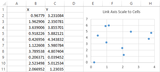
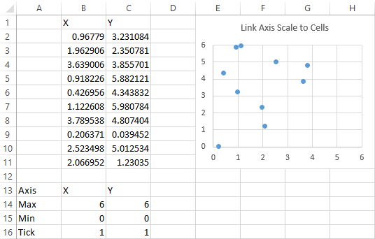
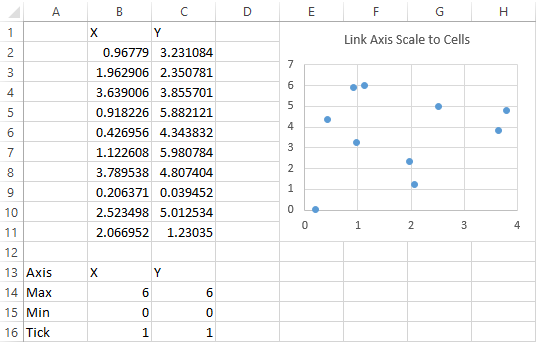 The cells B14:C16 can contain static values which the user can manually change, or they can contain formulas with your favorite axis scaling algorithms. See how to set up axis-scaling formulas in
 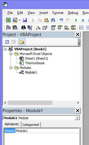 Double click on the module to open it. If there is no module, right click anywhere in the workbook’s project tree, choose Insert > Module. Or use Insert menu > Module. Up will pop a blank code module.
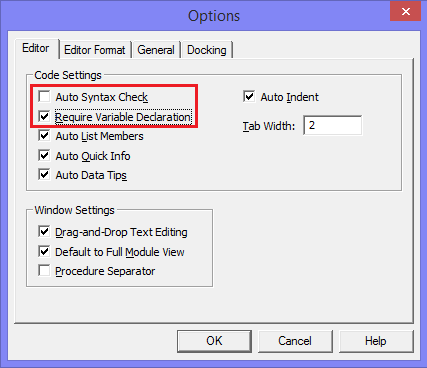
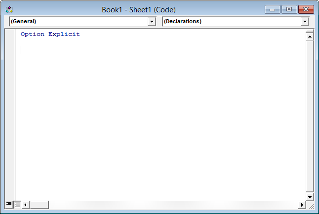
 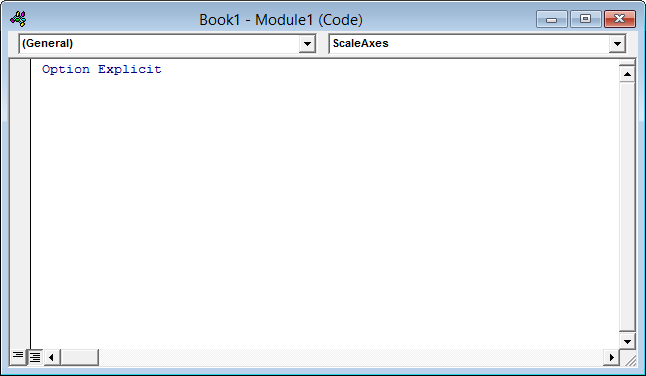 If your module does not say Option Explicit at the top, type it in manually. Then go to Tools > Options, and in the Editor tab check the Require Variable Declaration checkbox. This will place Option Explicit at the top of every new module, saving innumerable problems caused by typos. While in the Options dialog, uncheck “Auto Syntax Check”. This will save innumerable warnings about errors you already know about because the editor turns the font of the offending code red.
  You can use a simple procedure that changes the axes on demand. The following changes the scales of the active chart’s axes using the values in B14:C16. Select the chart, then run the code.
 Select the chart and run the code. You can run the code by pressing Alt+F8 to open the Macros dialog, selecting the procedure in the list of macros, and clicking Run.
  Or you could
 You can write the entire procedure yourself, but it’s easier and more reliable to let the VB Editor start it for you. Click on the left hand dropdown at the top of this module, and select Worksheet from the list of objects.
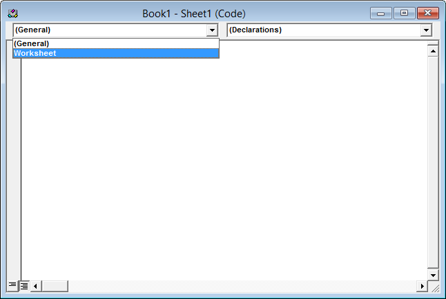 This places a stub for the Workbook_SelectionChange event in the module. Ignore this for now. Click on the right hand dropdown at the top of this module, and select Change from the list of events.
 You now have a couple event procedure stubs.
 Delete the Worksheet_SelectionChange stub, which we will not be needing, and type or paste the Worksheet_Change code into the Worksheet_Change stub.
 The code is given below, so you can copy it. When the event fires, it starts the procedure, passing in Target, which is the range that has changed. The procedure uses Select Case to determine which cell was changed, then changes the appropriate scale parameter of the appropriate axis.
