SERIES Formula

There are occasions when you may want to break the link between a chart and its underlying data. Maybe you copied the chart from another workbook, and you no longer have access to that workbook. Maybe you want to avoid the headaches that may arise from pasting a chart into PowerPoint or another program. Maybe you’re just tired of seeing this warning when you open the file:

There are several ways to disconnect your chart from its data source.

Chart Data

First let’s review chart data. I’ve written a lot about chart data, including

• Good Chart Data – The definitive description
• The Excel Chart SERIES Formula – also definitive
• Change Series Formula – Improved Routines
• How to Edit Series Formulas
• Simple VBA Code to Manipulate the SERIES Formula and Add Names to Excel Chart Series
• Edit Series Formulas

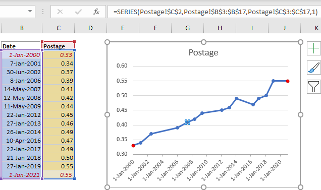
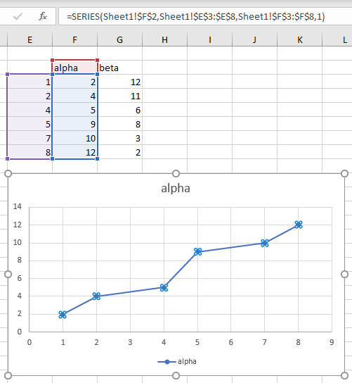
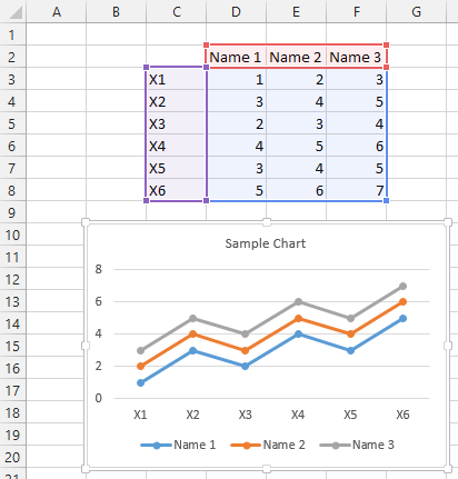
Below is a simple chart. A series is selected so the SERIES formula appears in the formula bar and the ranges in the formula are highlighted in the worksheet.

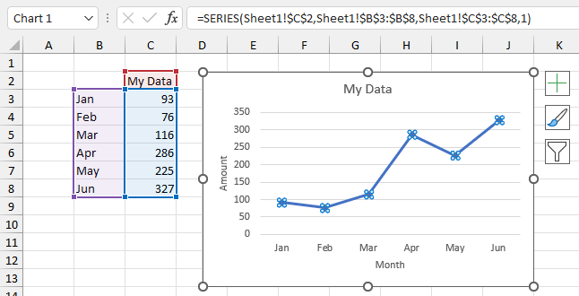
The SERIES formula looks like this:

=SERIES(Sheet1!$C$2,Sheet1!$B$3:$B$8,Sheet1!$C$3:$C$8,1)

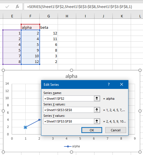
The arguments in the formula describe the sources of the data.

=SERIES(Series_Name,X_Values,Y_Values,Plot_Order)

• Series_Name can be a link to a worksheet range, text (enclosed in double quotes), or blank.
• X_Values can be a link to a worksheet range, an array enclosed in curly braces, or blank (and the chart will use 1, 2, 3, … for its X values).
• Y_Values can be a link to a worksheet range, or an array enclosed in curly braces.
• Plot_Order is an whole number between 1 and the number of series in the chart, signifying the order in which the series is drawn (complicated by chart type and axis group).

The cell addresses in the SERIES formula always use absolute references, such as $A$1, not relative references, like A1. But if you manually type relative references and press Enter, they will be converted to absolute references. The addresses always include the worksheet name.

If the chart links to data in another open Excel workbook, the SERIES formula includes the workbook name in square brackets before the worksheet name.

=SERIES('[Data Source.xlsm]Sheet1'!$C$2,'[Data Source.xlsm]Sheet1'!$B$3:$B$8,'[Data Source.xlsm]Sheet1'!$C$3:$C$8,1)

If the chart links to data in a closed Excel workbook, the SERIES formula includes the path, then the workbook name in square brackets, and finally the worksheet name.

=SERIES('C:\Long Path[Data Source.xlsx]Sheet1'!$C$2,'C:\Long Path[Data Source.xlsx]Sheet1'!$B$3:$B$8,'C:\Long Path[Data Source.xlsx]Sheet1'!$C$3:$C$8,1)

Copy a Picture of the Chart

One way to represent an unlinked chart is to copy a picture of the chart, then paste it where desired.

Select the chart, then on the Home tab of Excel’s ribbon, under the Copy dropdown, select Copy as Picture…

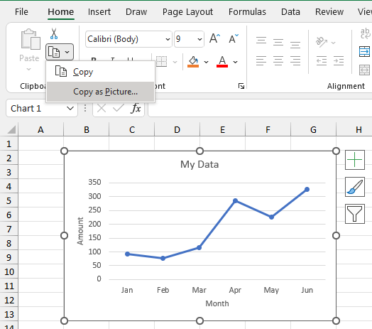
… then select the appropriate options (usually Bitmap instead of Picture; I haven’t been able to figure out the difference between on screen vs. as printed) …

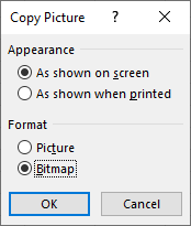
Then go to the other application, and Paste.

The disadvantage to this technique is that the pasted picture is no longer an Excel chart. You can no longer format any of the chart elements (rescale the axes, change marker styles or colors, etc.). Therefore, this method is unsuitable for use within Excel.

Change the Cell References to Hard-Coded Values

You can unlink chart data and still retain the actual chart with its formatting capabilities by editing the SERIES formula. Recall that the series formula in our first chart above was:

=SERIES(Sheet1!$C$2,Sheet1!$B$3:$B$8,Sheet1!$C$3:$C$8,1)

where the arguments referred to various links to the series data

=SERIES(Series_Name,X_Values,Y_Values,Plot_Order)

Select the series so that the SERIES formula appears in the formula bar, click in the formula bar so that the cursor is in the formula, and press F9. This keystroke converts references in the formula to their values:

=SERIES("My Data",{"Jan","Feb","Mar","Apr","May","Jun"},{93,76,116,286,225,327},1)

Series_Name becomes "MyData", X_Values becomes {"Jan","Feb","Mar","Apr","May","Jun"}, and Y_Values becomes {93,76,116,286,225,327}. Plot_Order is unchanged, of course, because it can only be a number, never a reference.

Press Esc to revert to the formula with references, or press Enter to keep the formula with hard-coded values.

If you select just one of the references in the formula, the F9 key only converts that reference to its value. These SERIES formulas are all valid:

=SERIES("My Data",Sheet1!$B$3:$B$8,Sheet1!$C$3:$C$8,1)
=SERIES(Sheet1!$C$2,{"Jan","Feb","Mar","Apr","May","Jun"},Sheet1!$C$3:$C$8,1)
=SERIES(Sheet1!$C$2,Sheet1!$B$3:$B$8,{93,76,116,286,225,327},1)
=SERIES(Sheet1!$C$2,{"Jan","Feb","Mar","Apr","May","Jun"},{93,76,116,286,225,327},1)

Automate with VBA

Any repetitive task that you can do manually, VBA can do faster with much less tedium.

Simple VBA Algorithm

To unlink chart data from all series in the active chart, simply run this code:

Sub DelinkChartFromData0()
  If ActiveChart Is Nothing Then
    MsgBox "Select a chart and try again", vbExclamation, "No Active Chart"
  Else
    Dim srs As Series
    For Each srs In ActiveChart.SeriesCollection
      ' Convert X Values to arrays of values
      srs.XValues = srs.XValues
      ' Convert Y Values to arrays of values
      srs.Values = srs.Values
      ' Convert series name to text
      srs.Name = srs.Name
    Next srs
  End If
End Sub

More Flexible Code

That’s nice enough, but I like to adjust a sub like this by including an argument, so I can pass in the object I want to process from any entry point. The function corresponding to this is

Sub DelinkChartFromData1(cht As Chart)
  Dim srs As Series
  For Each srs In cht.SeriesCollection
    ' Convert X Values to arrays of values
    srs.XValues = srs.XValues
    ' Convert Y Values to arrays of values
    srs.Values = srs.Values
    ' Convert series name to text
    srs.Name = srs.Name
  Next srs
End Sub

To process the active chart, I would call it with this entry point:

Sub DelinkActiveChartFromData1()
  If Not ActiveChart Is Nothing Then
    DelinkChartFromData1 ActiveChart
  End If
End Sub

To process all charts on the active sheet, I would use this:

Sub DelinkAllChartsFromData1()
  Dim chob As ChartObject
  For Each chob In ActiveSheet.ChartObjects
    DelinkChartFromData1 chob.Chart
  End If
End Sub

To select on or more charts to process, and ignore the rest, I use this approach:

Sub DelinkSelectedChartsFromData1()
  If Not ActiveChart Is Nothing Then
    DelinkChartFromData1 ActiveChart
  ElseIf TypeName(Selection) = "DrawingObjects" Then
    Dim shp As Shape
    For Each shp In Selection.ShapeRange
      If shp.HasChart Then
        DelinkChartFromData1 shp.Chart
      End If
    Next
  End If
End Sub

In fact, the last sub is all I need, since it does the active chart if there is one, replacing DelinkActiveChartFromData1, and it does any selected charts, so I could select all charts and run it to mimic DelinkAllChartsFromData1.

Fix the Date Axis

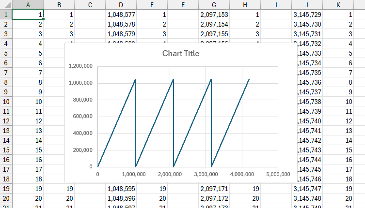
I was working on an example to show that it works for chart with lots of data points, and I happened to use dates as my X values.

I used DelinkSelectedChartsFromData1 and got the resulting chart.

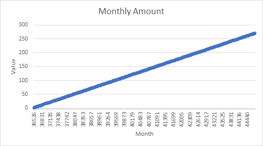
The SERIES formula is pretty long, but is nowhere near the limit (see Excel Chart Series Size Limits).

=SERIES("Value",{36526,36557,36586,36617,36647,36678,36708,36739,36770,36800,36831,36861,36892,36923,36951,36982,37012,37043,37073,37104,37135,37165,37196,37226,37257,37288,37316,37347,37377,37408,37438,37469,37500,37530,37561,37591,37622,37653,37681,37712,37742,37773,37803,37834,37865,37895,37926,37956,37987,38018,38047,38078,38108,38139,38169,38200,38231,38261,38292,38322,38353,38384,38412,38443,38473,38504,38534,38565,38596,38626,38657,38687,38718,38749,38777,38808,38838,38869,38899,38930,38961,38991,39022,39052,39083,39114,39142,39173,39203,39234,39264,39295,39326,39356,39387,39417,39448,39479,39508,39539,39569,39600,39630,39661,39692,39722,39753,39783,39814,39845,39873,39904,39934,39965,39995,40026,40057,40087,40118,40148,40179,40210,40238,40269,40299,40330,40360,40391,40422,40452,40483,40513,40544,40575,40603,40634,40664,40695,40725,40756,40787,40817,40848,40878,40909,40940,40969,41000,41030,41061,41091,41122,41153,41183,41214,41244,41275,41306,41334,41365,41395,41426,41456,41487,41518,41548,41579,4160
9,41640,41671,41699,41730,41760,41791,41821,41852,41883,41913,41944,41974,42005,42036,42064,42095,42125,42156,42186,42217,42248,42278,42309,42339,42370,42401,42430,42461,42491,42522,42552,42583,42614,42644,42675,42705,42736,42767,42795,42826,42856,42887,42917,42948,42979,43009,43040,43070,43101,43132,43160,43191,43221,43252,43282,43313,43344,43374,43405,43435,43466,43497,43525,43556,43586,43617,43647,43678,43709,43739,43770,43800,43831,43862,43891,43922,43952,43983,44013,44044,44075,44105,44136,44166,44197,44228,44256,44287,44317,44348,44378,44409,44440,44470,44501,44531,44562,44593,44621,44652,44682,44713},{1.59180141468432,2.98367529941487,3.53968832672474,4.166896463019,5.49680350931305,6.60295325255014,7.92084805050608,8.42969525036707,9.03114848703803,10.5276619316506,11.6955893543266,12.7967815520366,13.9389611218954,14.7527663401269,15.056329735329,16.5993323777924,17.3515548037874,18.5751579754327,19.5310520490484,20.1024924707731,21.0585061447489,22.5723596205116,23.6423776067453,24.1433918431237,25
.8809999743178,26.9737430334888,27.2520490776847,28.9524027272893,29.1845029748314,30.9521946135505,31.6902106518488,32.6795741650195,33.0489731513874,34.3260591677559,35.6901951915975,36.5728985726155,37.399073960589,38.3469907111962,39.9779540070637,40.6458619797685,41.8270884435173,42.4800724464723,43.5366272985535,44.8875676117536,45.2053138791033,46.1944737321369,47.3914095233474,48.8633128550379,49.5985742034472,50.7164885501005,51.653002976414,52.173798695412,53.797369677567,54.336065160202,55.2589150631074,56.4371639546982,57.3504724537478,58.7576090168706,59.8397486773469,60.5570284284911,61.2384044080596,62.8073951248627,63.0734139584437,64.023944739976,65.4569502217557,66.441196439216,67.8040167607499,68.4732296280772,69.383544349419,70.6736709532193,71.8772550111681,72.7285185169436,73.0304159679703,74.4543215360901,75.6139703970569,76.6795157883573,77.9474917376374,78.8675574588127,79.2434751623046,80.8059856927601,81.9149434410426,82.0822571567436,83.1165049108337,84.5766331546624,85.0485197930
954,86.4516756787662,87.103472072234,88.6166607931416,89.5569751902823,90.2997637601853,91.4861009853597,92.738947366043,93.1212971468925,94.0166978760269,95.1888503720746,96.8377506737342,97.3036391294494,98.126217895739,99.339467893605,100.259054804445,101.840983590986,102.741718964783,103.082626950564,104.362149881911,105.760866364373,106.396030094412,107.226463877175,108.638218224396,109.379526574316,110.109027223762,111.420326031626,112.61771263781,113.468694206656,114.619213431217,115.278679680971,116.466011457757,117.537068146506,118.753523891166,119.704656141103,120.131070166454,121.822525894342,122.977159915521,123.640235472236,124.383000359254,125.608871736392,126.188489945214,127.414144604553,128.39601244846,129.115889297518,130.08797401699,131.159077879218,132.410010962127,133.535396508137,134.718791752223,135.443733080568,136.661870239714,137.29210822438,138.55656753413,139.308552070942,140.27987742426,141.456569779806,142.774325544055,143.243355927806,144.505167482867,145.111184143168,146.30748
3083571,147.464847220224,148.218427246658,149.769670436945,150.776656088281,151.515371748972,152.408346863735,153.29435331721,154.857749604455,155.212400832703,156.31398296817,157.430827877581,158.068214294863,159.246613771057,160.346285238108,161.703341756362,162.939983684318,163.581827103078,164.41963298477,165.632147153497,166.697413290467,167.83618109404,168.878480595484,169.817382059171,170.125826262302,171.174106119149,172.182319412083,173.683778271622,174.350253903931,175.280205756401,176.628020353313,177.602771096537,178.468667385597,179.645508668238,180.131396317678,181.258745156011,182.238164094744,183.821618545389,184.261328363069,185.932899850116,186.187494356367,187.586391685274,188.120772297618,189.794395110081,190.509727284739,191.179753691424,192.54771311589,193.831688905835,194.638416224214,195.906316127413,196.845527552348,197.02489756276,198.382679905726,199.860935825007,200.422827058144,201.110300744418,202.209577950068,203.499633489411,204.12638600329,205.314473205528,206.095829209215,20
7.070675561553,208.875077186077,209.071848934263,210.37641200788,211.34927750657,212.666535668482,213.400957572161,214.438684951166,215.464275837814,216.580366174425,217.797909408301,218.167376086905,219.366623356776,220.548163602681,221.316902416248,222.044068195978,223.356501739512,224.984206101239,225.14746583972,226.275382045765,227.310864151405,228.851337545147,229.175137589426,230.520419824664,231.361806010337,232.175186942816,233.450560796329,234.269397102542,235.272652848491,236.560089595496,237.571235289495,238.499139612489,239.133135844129,240.582849816789,241.827775202926,242.833982805547,243.988020788098,244.077263106469,245.085954088788,246.671199871053,247.086129757983,248.030390822573,249.043987276631,250.071893428251,251.525524796095,252.600631102785,253.754358498755,254.665241202158,255.625959629045,256.98261131318,257.320204395814,258.444509485282,259.533974191495,260.492799645349,261.603579334917,262.194476107706,263.615554634444,264.987806666296,265.830581271325,266.39664304882,267.294282
876198,268.348630086833,269.253293622165,270.082557692269},1)

Unfortunately, the X axis tick labels have lost their date formatting. In the sub, the srs.XValues = srs.XValues converted the input dates into numbers, because internally Excel stores dates as the number of days since 1 January 1900. Easy enough to apply the date format manually.

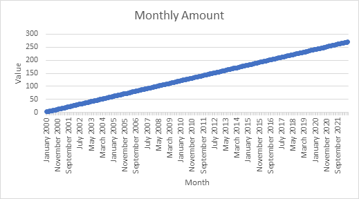
Apparently, the nice spacing that comes with an actual date axis is gone. The chart above has dates, but the axis is a simple category axis. I’ll have to adjust the procedure to prevent a date axis from being changed into a category axis. Before I convert the links to values, I will apply the number format to the axis ticks. Then if it is a date axis, I will make sure the chart treats it as one; this is complicated by the fact that Excel often applies the date category type automatically based on the data.

Sub DelinkChartFromData2(cht As Chart)
  Dim iGrp As XlAxisGroup
  For iGrp = xlPrimary To xlSecondary
    Dim ax As Axis
    Set ax = cht.Axes(xlCategory, iGrp)
    With ax
      ' apply formats
      .TickLabels.NumberFormat = .TickLabels.NumberFormat
      If IsDateAxis(ax) Then
        ' apply date type
        ax.CategoryType = xlTimeScale
      End If
    End With
  Next
  Dim srs As Series
  For Each srs In cht.SeriesCollection
    ' Convert X Values to arrays of values
    srs.XValues = srs.XValues
    ' Convert Y Values to arrays of values
    srs.Values = srs.Values
    ' Convert series name to text
    srs.Name = srs.Name
  Next srs
End Sub

This function tests whether an axis is a date category type. The BaseUnit property is undefined unless the axis is a date axis.

Function IsDateAxis(ax As Axis) As Boolean
  If ax.Type = xlCategory Then
    Dim vTest As Variant
    On Error Resume Next
    vTest = ax.BaseUnit
    IsDateAxis = (Err.Number = 0)
    On Error GoTo 0
  End If
End Function

The corresponding entry point that I call the above with is familiar:

Sub DelinkSelectedChartsFromData2()
  If Not ActiveChart Is Nothing Then
    DelinkChartFromData2 ActiveChart
  ElseIf TypeName(Selection) = "DrawingObjects" Then
    Dim shp As Shape
    For Each shp In Selection.ShapeRange
      If shp.HasChart Then
        DelinkChartFromData2 shp.Chart
      End If
    Next
  End If
End Sub

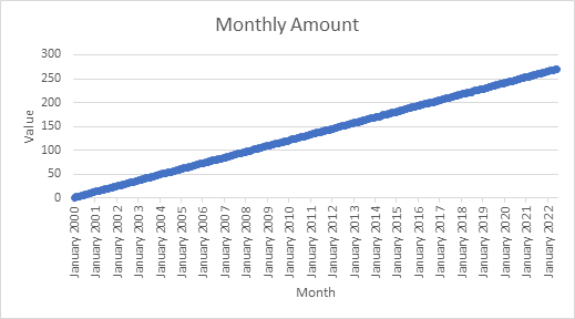
The resulting chart is now indistinguishable from the original:

Unlink the Chart and Axis Titles

It’s easy to link many of a chart’s text elements to a worksheet range. Select the text element, click in the formula bar, type = and click on the cell or range containing the text you want displayed. The result is a link formula like =Sheet1!$A$1, and the text element updates dynamically to display whatever is in the reference. This works for the chart title, axis titles, data labels, and textboxes and other shapes that contain text.

If you’re delinking the chart’s data, you probably want to delink the titles in the chart. A simple VBA routine to do just that is shown below. For each possible title, see if the formula begins with an equals sign (if not, the formula just shows the text), and if so, replace the title’s text with the title’s text.

Sub UnlinkTitles()
  If Not ActiveChart Is Nothing Then
    With ActiveChart
      If .HasTitle Then
        If Left$(.ChartTitle.Formula, 1) = "=" Then
          ' convert chart title link to text
          .ChartTitle.Text = .ChartTitle.Text
        End If
      End If
      Dim iAx As XlAxisGroup
      For iAx = xlCategory To xlSeriesAxis
        Dim iGrp As XlAxisType
        For iGrp = xlPrimary To xlSecondary
          If .HasAxis(iAx, iGrp) Then
            With .Axes(iAx, iGrp)
              If .HasTitle Then
                If Left$(.AxisTitle.Formula, 1) = "=" Then
                  ' convert axis title link to text
                  .AxisTitle.Text = .AxisTitle.Text
                End If
              End If
            End With
          End If
        Next
      Next
    End With
  End If
End Sub

Let’s merge this into our last Delink The Chart routine (I’ve also included the test for a date axis:

Sub DelinkChartFromData3(cht As Chart)
  With cht
    If .HasTitle Then
      If Left$(.ChartTitle.Formula, 1) = "=" Then
        ' convert chart title link to text
        .ChartTitle.Text = .ChartTitle.Text
      End If
    End If
    Dim iAx As XlAxisType
    For iAx = xlCategory To xlSeriesAxis
      Dim iGrp As XlAxisGroup
      For iGrp = xlPrimary To xlSecondary
        If .HasAxis(iAx, iGrp) Then
          Dim ax As Axis
          Set ax = .Axes(iAx, iGrp)
          With ax
            If .HasTitle Then
              If Left$(.AxisTitle.Formula, 1) = "=" Then
                ' convert axis title link to text
                .AxisTitle.Text = .AxisTitle.Text
              End If
            End If
            If iAx = xlCategory Then
              ' apply formats
              .TickLabels.NumberFormat = .TickLabels.NumberFormat
              If ax.Type = xlCategory Then
                Dim vTest As Variant
                On Error Resume Next
                vTest = ax.BaseUnit
                If (Err.Number = 0) Then
                  ' apply date type
                  ax.CategoryType = xlTimeScale
                End If
                On Error GoTo 0
              End If
            End If
          End With
        End If
      Next
    Next
    Dim srs As Series
    For Each srs In .SeriesCollection
      ' Convert X Values to arrays of values
      srs.XValues = srs.XValues
      ' Convert Y Values to arrays of values
      srs.Values = srs.Values
      ' Convert series name to text
      srs.Name = srs.Name
    Next srs
  End With
End Sub

And we’ll call it using the familiar entry point:

Sub DelinkSelectedChartsFromData3()
  If Not ActiveChart Is Nothing Then
    DelinkChartFromData3 ActiveChart
  ElseIf TypeName(Selection) = "DrawingObjects" Then
    Dim shp As Shape
    For Each shp In Selection.ShapeRange
      If shp.HasChart Then
        DelinkChartFromData3 shp.Chart
      End If
    Next
  End If
End Sub