I recently wrote about how I wrote an Excel Lambda Moving Average formula. I started with internet searches, which led to formulas which didn’t work or formulas which were too complicated for me to understand. After a brief and amusing foray into ChatGPT, I built myself a workable formula that worked by generating a running sum, subtracting an earlier point’s running sum from the current point’s running sum, and dividing by the number of points. This worked fine for a simple N-point moving average, but it broke down for N-day moving averages where some days in the data set may be missing. And there are probably better ways to do the moving average without calculating running sums.
Jon’s Previous Moving Average Formula
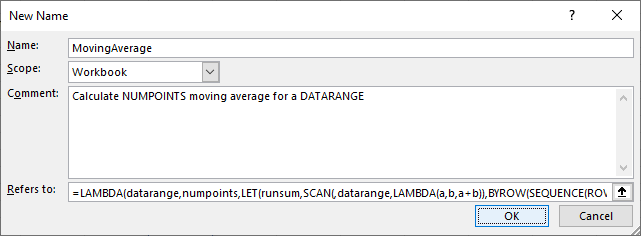
I developed the following LAMBDA moving average formula, as described in my previous post:
=LAMBDA(datarange,numpoints,
  LET(
    runsum,SCAN(,datarange,LAMBDA(a,b,a+b)),
    BYROW(
      SEQUENCE(ROWS(datarange)),
      LAMBDA(x,
      IF(
        x<numpoints,
        NA(),
        (INDEX(runsum,x)-IF(x=numpoints,0,INDEX(runsum,x-numpoints)))
        /numpoints)
      )
    )
  )
)
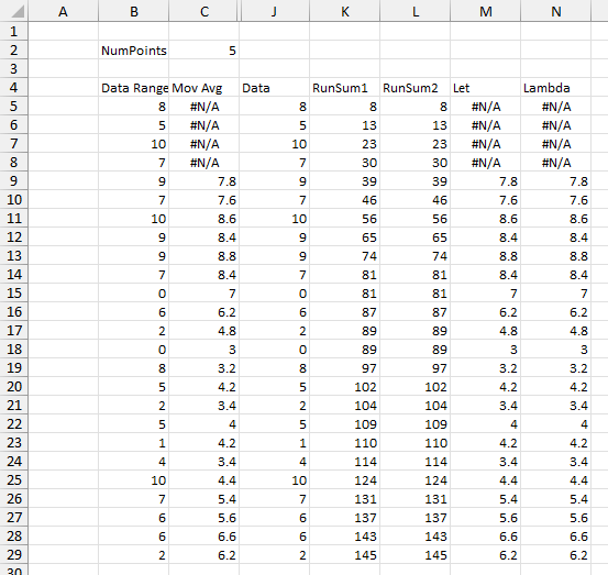
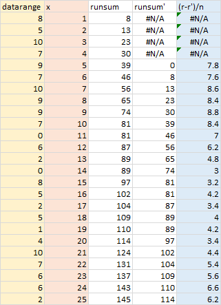
Let me partially deconstruct the formula below, showing internal calculations leading to the moving average. The LAMBDA takes the data range and numpoints, the number of points in the moving average, as arguments. The first column contains 25 values in the data range. Column 2 is the element number x of the output array which is created using BYROW. The third column contains the running sum, created using SCAN. The fourth column is the same running sum offset by numpoints. The fifth column shows the moving average calculation, which is the running sum minus the running sum numpoints points ago divided by numpoints. Where x is less than numpoints, the result is #N/A, because there aren’t enough points to divide by numpoints. Where x equals numpoints, zero is subtracted from the running sum, since the running sum of zero points is zero.
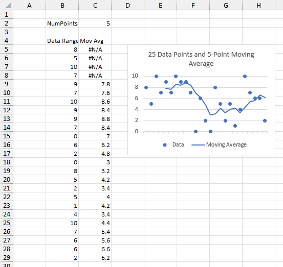
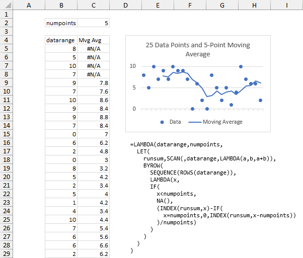
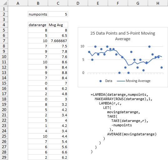
Here is how it looks in action. The data range is in B5:B29, the number of points being averaged is in C2, and the moving range formula is entered into cell C5 and spills down to C29. The first several calculated values are #N/A, until we have as many points as we are averaging (the number in C2).
Improvement #1: CHOOSEROWS
I exchanged several comments on my earlier post with a smart reader named Henk-Jan van Well, who suggested several improvements to the moving average algorithm, starting with CHOOSEROWS.
CHOOSEROWS allows you to select which rows of an array to use. CHOOSEROWS(array,3) returns the 3rd row of that array. CHOOSEROWS(array,{2,4}) returns the 2nd and 4th rows. Our approach uses SEQUENCE to generate a list of row numbers to return, and we simply use AVERAGE to, well, average these rows.
=LAMBDA(datarange,numpoints,
  MAKEARRAY(
    ROWS(datarange),,
    LAMBDA(r,c,
      IF(
        r<numpoints,
        NA(),
        AVERAGE(
          CHOOSEROWS(
            datarange,
            SEQUENCE(numpoints,,1+r-numpoints)
          )
        )
      )
    )
  )
)
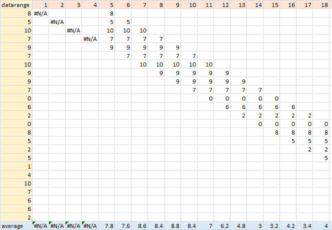
Here is a deconstruction of the formula. Again, the LAMBDA moving average takes the data range and numpoints, the number of points in the moving average, as arguments. The data range is in the first column, the output row number r is in the first row (I’m only showing the first 18 points, but you get the idea). For the first 4 points (less than numpoints), the function returns #N/A. After that, CHOOSEROWS selects the indicated values from the data range. These are averaged in the last row, which is returned by the function.
The calculations and chart look the same as above.

Improvement #2: Calculate Averages for First Points
Henk-Jan also mentioned an averaging scheme used by some econometricians for points that occur before the official number of points to average. I don’t like that definition of averaging early points, but I have an alternative, which simply averages however many points there are. This actually simplifies our formula.
=LAMBDA(datarange,numpoints,
  MAKEARRAY(
    ROWS(datarange),,
    LAMBDA(
      r,c,
      AVERAGE(
        CHOOSEROWS(
          datarange,
          SEQUENCE(
            MIN(r,numpoints),,
            MAX(1,1+r-numpoints)
          )
        )
      )
    )
  )
)
Here is a deconstruction of the new formula. The LAMBDA takes the data range and numpoints as arguments. The data range is in the first column, the output row number r is in the first row (only showing the first 18 points). CHOOSEROWS selects the indicated values from the data range; note that fewer than numpoints are selected for the first few columns. The selected values are averaged in the last row, which is returned by the function.
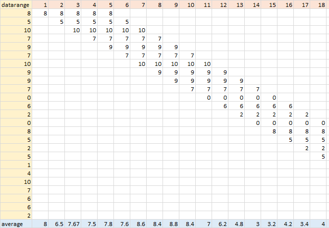
The results look the same as before, except that the moving average begins right at the first point.

Improvement #3: TAKE and DROP
The array functions TAKE and DROP allow you to keep or remove rows and columns from the beginning and end of an array. This is simpler than generating a list of row numbers to pass into CHOOSEROWS to define a moving array to average.
For each row r of the moving average array we create, we TAKE the first r rows, then we DROP all but numpoints from the beginning (and if r is less than numpoints, we don’t DROP any rows).
=LAMBDA(datarange,numpoints,
  MAKEARRAY(ROWS(datarange),1,
    LAMBDA(r,c,
      LET(
        movingdatarange,
        DROP(
          TAKE(datarange,r),
          MAX(0,r-numpoints)
         ),
        AVERAGE(movingdatarange)
      )
    )
  )
)
I’ve only deconstructed a few points below. The LAMBDA moving average takes the data range (which is r rows tall) and numpoints as arguments. The function uses TAKE to take the first r rows, then uses DROP to drop the first r–numpoints rows, or zero if r<numpoints. For point 3, the function takes the first 3 rows, then drops zero rows, and returns the average of these three values. For point 10, the function takes the first 10 rows, drops 5 rows (r–numpoints = 10-5), and averages these 5 (numpoints) rows. For point 23, the function takes the first 23 rows, drops 18 rows (r–numpoints = 23-5), and averages these 5 (numpoints) rows.
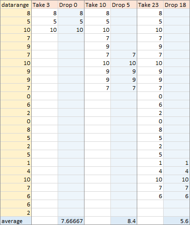
The result looks the same, with the moving range starting right at the beginning. The LAMBDA formula may be a bit shorter, but it also seems more reliable when the number of points may vary (as when averaging by dates below).

An easier alternative is the following, where we TAKE the first r rows for each array element, then TAKE the last numpoints rows of this. If you try to TAKE more than the number of rows in an array, you simply get the entire array.
=LAMBDA(datarange,numpoints,
  MAKEARRAY(ROWS(datarange),1,
    LAMBDA(r,c,
      LET(
        movingdatarange,
        TAKE(
          TAKE(datarange,r),
          -numpoints
         ),
        AVERAGE(movingdatarange)
      )
    )
  )
)
Again I’ve only deconstructed a few points below. The LAMBDA takes the data range (which is r rows tall) and numpoints as arguments. The function uses TAKE to take the first r rows, then uses TAKE again to take the last numpoints rows; if r<numpoints then TAKE only takes as many rows as are available. For point 3, the function takes the first 3 rows, then takes all available rows, and returns the average of these three values. For point 10, the function takes the first 10 rows, takes the last 5 (numpoints) of these rows, and averages these rows. For point 23, the function takes the first 23 rows, then keeps the last 5 (numpoints) of these rows, and averages these rows.
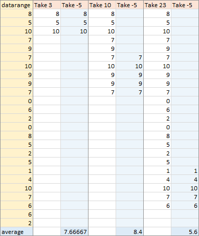
Same results, but the function is a few characters shorter and may be easier to understand.
Major Enhancement: Moving Average by Date
If a range has values for all dates, then a moving average by date is the same as a moving average by point. A seven-day moving average is a seven-point moving average. But if some dates are missing, then a seven-point moving average will average points from more than seven days. I want to average only data which falls within a seven-day window, which means averaging fewer than seven points if some days are missing. The screenshot below illustrates the problem. There will be a missing value when a measurement is not made on a given day. Note for example, that 1/9/2023 and 1/10/2023 are missing.
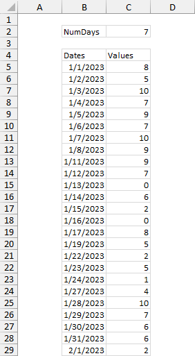
Here is the LAMBDA formula, which takes the dates, the data values to be averaged, and numdays, the number of days to average, as inputs.
=LAMBDA(daterange,datarange,numdays,
  MAKEARRAY(ROWS(datarange),1,
    LAMBDA(r,c,
      LET(
        firstdate,
        XMATCH(
          INDEX(daterange,r)-numdays+1,
          daterange,
          1),
        movingdatarange,
        DROP(
          TAKE(datarange,r),
          MAX(0,firstdate-1)
        ),
        AVERAGE(movingdatarange)
      )
    )
  )
)
In the first section of the deconstruction below I show row number (tan-shaded), the end date for that average, which is the date for that row number, the allowed start date, which is the end date minus numdays+1, and the actual start date, which is the earliest date on or after the allowed start date. The blue shaded dates show which rows have different allowed and actual start dates.
In the second section of the deconstruction, I show dates (gold-shaded) and values in the first two columns. In the first row is the row number r of the output array (tan-shaded). The remaining columns show the dates that fall between the allowed start date and end date for each row. The green-shaded columns show which columns contain fewer than numdays dates. Not very many of the rows actually average numdays values.
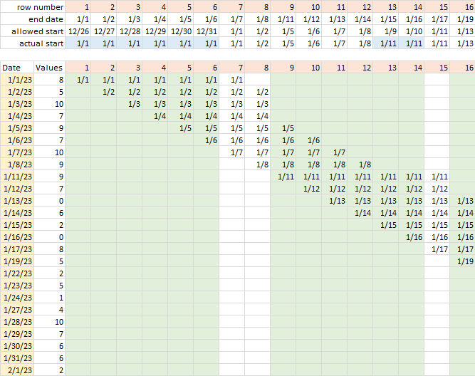
The LAMBDA moving average formula uses the TAKE/DROP approach from the previous section to average the appropriate values.
Below is the output of the formula.
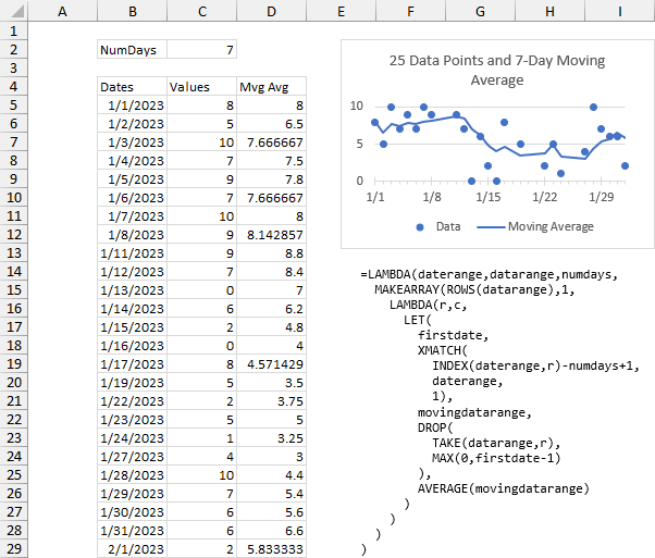
Here is comparison of a 7-point (orange line) and a 7-day (blue line) moving average. The blue shaded cells show where the two are not the same.

This is the case when I track my weight: while traveling or when I wake up too late or am just too busy in the morning to weigh myself, then I don’t have a row for the date I’ve missed. This formula treats such occasions nicely.
Sample Workbook
You can click on this link to download a workbook that contains these examples: Improved Excel Lambda Moving Average.xlsx.
More Articles About Dynamic Arrays, LET, and LAMBDA
- ISPRIME Lambda Function
- Lambda Moving Average Formulas
- Excel Lambda Moving Average
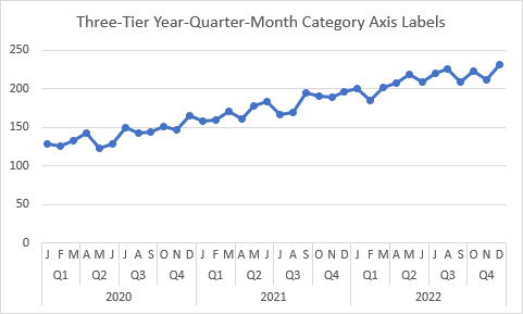
- LAMBDA Function to Build Three-Tier Year-Quarter-Month Category Axis Labels
- Dynamic Array Histogram
- Calculate Nice Axis Scales with LET and LAMBDA
- VBA Test for New Excel Functions
- Dynamic Arrays, XLOOKUP, LET – New Excel Features


