Calculating “Nice” Axis Scales
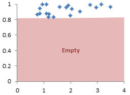
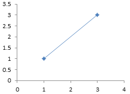
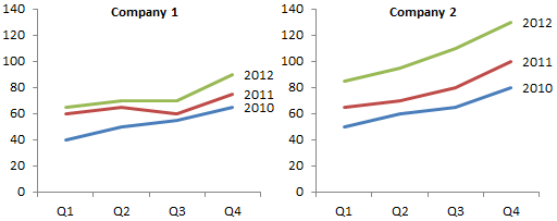
“Nice” axis scales allow all of your data to be shown, and depending on chart type, improve resolution by minimizing white space between plotted data and the edges of the chart. These scales also allow for a reasonable number of tick marks and gridlines, and have tick marks at human-friendly intervals. A friendly scale is 20-25-30-35-40; an unfriendly scale is 17-24-31-38.
I’ve written before about how you can Calculate Nice Axis Scales in Your Excel Worksheet and Calculate Nice Axis Scales in Excel VBA. The problem with the first of these is that it requires setting up a block of cells do do intermediate calculations, and the problem with the second is that, well, it uses VBA. VBA is supported only for Windows and Mac, not online or mobile, and its use raises security concerns.
LET, LAMBDA, and Dynamic Arrays
New features in Microsoft 365 (a/k/a Office 365) give us the flexibility of VBA functions, but allow the formulas to reside in the worksheet, using worksheet functions. In this tutorial I will make use of LET, LAMBDA, and Dynamic Arrays.
I’ve cleaned up the workbook I used for this exercise, and you can download it from this link:
Calculate Nice Axis Scales with LET and LAMBDA.xlsx
The LET Function
The LET function allows you to define names in the formula for values or intermediate calculations. The syntax is:
=LET(Name1,NameValue1,Result)
=LET(Name1,NameValue1,Name2,NameValue2,...,Result)
Each name must begin with a letter but not look like a cell reference (e.g., ABCD123 is valid, but A1 is not). Each name value as well as the result can be a cell reference (A1 is allowed here), a constant (3.14159), or a calculation (2*Input). You can specify up to 126 pairs of names and name values.
A couple illustrations:
=LET(Input,A1,2*Input)
=LET(Side1,A1,Side2,A2,SQRT(Side1^2+Side2^2))
=LET(Side1,A1,Side2,A2,SumSquares,Side1^2+Side2^2,SQRT(SumSquares))
These LET formulas are more complicated than a regular formula would be, but LET allows a given value to be looked up or calculated once and reused in the calculation.
LET was introduced several months ago, and has now propagated out to all Microsoft 365 subscribers.
The LAMBDA Function
The LAMBDA function is similar to LET, and can incorporate LET, but it is much more powerful. You define inputs and intermediate calculations, and output a result. Syntax:
=LAMBDA(ParameterOrCalculation1,ParameterOrCalculation2,...)
You can specify up to 253 parameters.
Repeating the illustrations above:
=LAMBDA(Input,2*Input)
=LAMBDA(Side1,Side2,SQRT(Side1^2+Side2^2))
=LAMBDA(Side1,Side2,LET(SumSquares,Side1^2+Side2^2,SQRT(SumSquares)))
You can’t use these as shown in the worksheet. You must either define a name using the LAMBDA formula as its definition, then call it from the worksheet, or you can enter the LAMBDA followed by a comma-delimited list of parameters in parentheses.
So I can define a name called DoubleFunction, using the first LAMBDA formula above, and call it in the worksheet like this:
=DoubleFunction(A1)
You can define another Name, call it Hypotenuse, and use the second or third LAMBDA formulas, and call it like this:
=Hypotenuse(A1,A2)
Alternatively, the first LAMDBA formula above can be used in a worksheet cell like this:
=LAMBDA(Input,2*Input)(A1)
and the second like this:
=LAMBDA(Side1,Side2,SQRT(Side1^2+Side2^2))(A1,A2)
Using LAMBDAs in the worksheet isn’t useful by itself, though it makes it easy to test your formulas before using them to define a Name. And if you forget to append the parameters to the formula, you will get a #CALC! error in the cell.
You unleash the power of LAMBDAs when you use one in a Name, because you can then use this as a function anywhere in the workbook, without repeating the function each time. When the formula needs to be modified, it only needs to be modified in the Name definition, not in each place it is used, so each time it is used, it uses the same formula.
LAMBDA has been introduced to Office Insiders, so regular Microsoft 365 subscribers will have to wait a few months or so.
Dynamic Arrays
Dynamic Arrays have now been part of Microsoft 365 for some time. These formulas provide many great capabilities, and the internet is loaded with great examples. I will use them to output three values (axis minimum, axis maximum, and axis major unit) using only one formula.
I can use CHOOSE to convert separate values into a Dynamic Array. The syntax is:
=CHOOSE(index_num,value1,value2,value3,…)
If index_num is 1, CHOOSE returns value1, in index_num is 2, it returns value2, etc. If I enter an array of values for index_num, CHOOSE returns an array, as follows:
=CHOOSE({1;2},Value1,Value2)
returns a vertical array of Value1 and Value2, because {1;2} is a vertical array.

In the same way,
=CHOOSE({1,2},Value1,Value2)
returns a horizontal array of Value1 and Value2, because {1,2} is a horizontal array .

Alternatively, I can wrap my function in TRANSPOSE() to convert a vertical array to horizontal. This is the better approach, so I only need to create one function to produce my output, and I can use TRANSPOSE only if I need that output in a horizontal array.
=CHOOSE({1;2},Value1,Value2)

When I compute my axis scales, I usually output them in a column of two or three cells.
Calculating Axis Scales with LET and LAMBDA
Algorithm
The algorithm to calculate axis scales has a few parts. First, we need to check that the minimum is in fact less than the maximum, and if not, switch them; if the minimum and maximum are the same, we need to move them away from each other.
Given appropriate minimum and maximum values, we need to move them slightly further apart to ensure that there is a small margin between all points and the edges of the plot area.
Finally, given the magnitudes of these values, we need to select an appropriate major scale unit (tick spacing), then find the minimum and maximum axis scale values that are a multiple of the major scale unit.
Sort Min and Max
Using names min_0 and max_0 for the inputs in A1 and A2, I can use this LET formula to list the inputs in ascending order, :
=LET(min_0,A1,max_0,A2,CHOOSE({1;2},MIN(min_0,max_0),MAX(min_0,max_0)))
I can use this LAMBDA in the worksheet to get the same result:
=LAMBDA(min_0,max_0,CHOOSE({1;2},MIN(min_0,max_0),MAX(min_0,max_0)))(A1,A2)
Or I can define a Name (Formula tab > Define Name), enter a function name like MinMax0, and enter this formula in the Refers To box:
=LAMBDA(min_0,max_0,CHOOSE({1;2},MIN(min_0,max_0),MAX(min_0,max_0)))
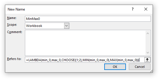
Editing formulas in the Define Name dialog is no fun, since the box is small and there is no IntelliSense. But once you have it working in the worksheet with the arguments in parentheses at the end, you can just paste in the formula.
The best part is that you can now use this function anywhere, like this:
=MinMax0(A1,A2)
Sort Min and Max – Better Way
Since I want to use the adjusted min and max in subsequent calculations, I want them in the form of additional names within the formulas. This means I’ll have to use LET within my LAMBDA.
In my LET formula, I’ll introduce two new names, min_1 and min_2 for the intermediate calculations:
=LET(min_0,A1,max_0,A2,min_1,MIN(min_0,max_0),max_1,MAX(min_0,max_0),CHOOSE({1;2},min_1,max_1))
These formulas are getting longer, but you can accommodate them in the Formula Bar. You can type Alt+Enter to insert a new line in the formula, then pad each line with space characters to provide indenting.
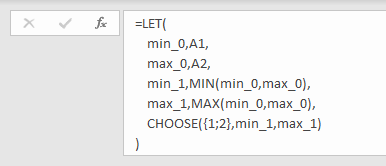
My LAMBDA with the nested LET looks like this in the worksheet:
=LAMBDA(min_0,max_0,LET(min_1,MIN(min_0,max_0),max_1,MAX(min_0,max_0),CHOOSE({1;2},min_1,max_1)))(A1,A2)
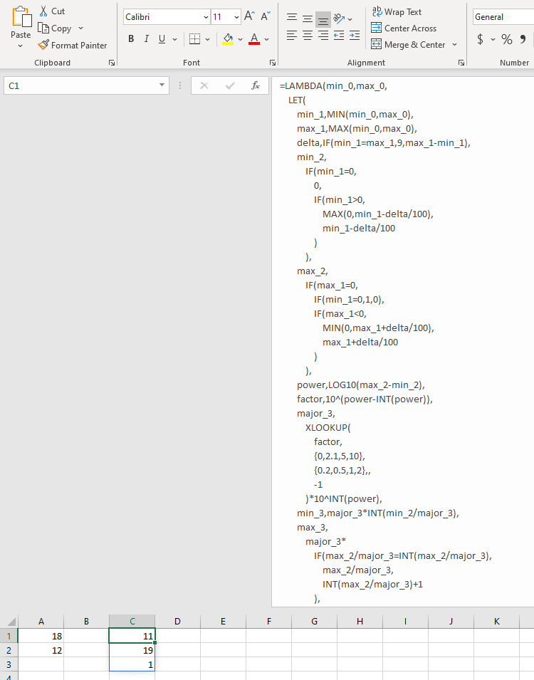
Here it is nicely formatted in the Formula Bar:
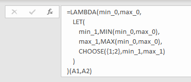
And I can define a new Name called MinMax1 that refers to this LAMBDA:
=LAMBDA(min_0,max_0,LET(min_1,MIN(min_0,max_0),max_1,MAX(min_0,max_0),CHOOSE({1;2},min_1,max_1)))
And I call it like this:
=MinMax1(A1,A2)
Adjust Min and Max
Now I can adjust my sorted minimum and maximum values to allow for a small margin, while also adjusting for equal min and max values. I need to add names min_2 and max_2 for the extended calculations.
Here is my new LET formula:
=LET(min_0,A1,max_0,A2,min_1,MIN(min_0,max_0),max_1,MAX(min_0,max_0),min_2,IF(min_1=0,0,IF(min_1>0,MAX(0,min_1-(max_1-min_1)/100),min_1-(max_1-min_1)/100)),max_2,IF(max_1=0,IF(min_1=0,1,0),IF(max_1<0,MIN(0,max_1+(max_1-min_1)/100),max_1+(max_1-min_1)/100)),CHOOSE({1;2},min_2,max_2))
or if it’s easier to read:
=LET(min_0,A1,max_0,A2,min_1,MIN(min_0,max_0),max_1,MAX(min_0,max_0),min_2,IF(min_1=0,0,IF(min_1>0,MAX(0,min_1-(max_1-min_1)/100),min_1-(max_1-min_1)/100)),max_2,IF(max_1=0,IF(min_1=0,1,0),IF(max_1<0,MIN(0,max_1+(max_1-min_1)/100),max_1+(max_1-min_1)/100)),CHOOSE({1;2},min_2,max_2))
My new LAMBDA:
=LAMBDA(min_0,max_0,LET(min_1,MIN(min_0,max_0),max_1,MAX(min_0,max_0),min_2,IF(min_1=0,0,IF(min_1>0,MAX(0,min_1-(max_1-min_1)/100),min_1-(max_1-min_1)/100)),max_2,IF(max_1=0,IF(min_1=0,1,0),IF(max_1<0,MIN(0,max_1+(max_1-min_1)/100),max_1+(max_1-min_1)/100)),CHOOSE({1;2},min_2,max_2)))(A1,A2)
or
=LAMBDA(min_0,max_0,LET(min_1,MIN(min_0,max_0),max_1,MAX(min_0,max_0),min_2,IF(min_1=0,0,IF(min_1>0,MAX(0,min_1-(max_1-min_1)/100),min_1-(max_1-min_1)/100)),max_2,IF(max_1=0,IF(min_1=0,1,0),IF(max_1<0,MIN(0,max_1+(max_1-min_1)/100),max_1+(max_1-min_1)/100)),CHOOSE({1;2},min_2,max_2)))(A1,A2)
I can define a Name called MinMax2 that uses this LAMBDA, without the trailing (A1,A2).
The Finished Functions
I need to take the latest calculations, perform some intermediate calculations using names delta, power, and factor, do a quick lookup, then calculate min_3, max_3, and major_3 to be output into a three-cell vertical array.
The final LET:
=LET(min_0,A1,max_0,A2,min_1,MIN(min_0,max_0),max_1,MAX(min_0,max_0),delta,IF(min_1=max_1,9,max_1-min_1),min_2,IF(min_1=0,0,IF(min_1>0,MAX(0,min_1-delta/100),min_1-delta/100)),max_2,IF(max_1=0,IF(min_1=0,1,0),IF(max_1<0,MIN(0,max_1+delta/100),max_1+delta/100)),power,LOG10(max_2-min_2),factor,10^(power-INT(power)),major_3,XLOOKUP(factor,{0,2.1,5,10},{0.2,0.5,1,2},,-1)*10^INT(power),min_3,major_3*INT(min_2/major_3),max_3,major_3*IF(max_2/major_3=INT(max_2/major_3),max_2/major_3,INT(max_2/major_3)+1),CHOOSE({1;2;3},min_3,max_3,major_3))
And the final LAMBDA:
=LAMBDA(min_0,max_0,LET(min_1,MIN(min_0,max_0),max_1,MAX(min_0,max_0),delta,IF(min_1=max_1,9,max_1-min_1),min_2,IF(min_1=0,0,IF(min_1>0,MAX(0,min_1-delta/100),min_1-delta/100)),max_2,IF(max_1=0,IF(min_1=0,1,0),IF(max_1<0,MIN(0,max_1+delta/100),max_1+delta/100)),power,LOG10(max_2-min_2),factor,10^(power-INT(power)),major_3,XLOOKUP(factor,{0,2.1,5,10},{0.2,0.5,1,2},,-1)*10^INT(power),min_3,major_3*INT(min_2/major_3),max_3,major_3*IF(max_2/major_3=INT(max_2/major_3),max_2/major_3,INT(max_2/major_3)+1),CHOOSE({1;2;3},min_3,max_3,major_3)))(A1,A2)
While it’s easier to read in expanded form, this last one doesn’t even fit on my large secondary monitor. It’s only about 500 characters, though, and Excel’s limit is 8192 characters in a formula.
That last LAMBDA can be used to define a Name called MinMax3, but I decided that MinMaxMajor is a better name.
Further Work
The next thing I want to try is to refactor this last LAMBDA function into several smaller ones. The first will convert the separate inputs into an array, the second will ensure the values in the array are sorted, the third will add the small margins, the fourth will perform the XLOOKUP, and the fifth will compute the axis scale parameters.
But my brain is tired, so I’ll do this another day.
More Axis Scale Articles
- Calculate Nice Axis Scales with LET and LAMBDA
- Calculate Nice Axis Scales in Your Excel Worksheet
- Calculate Nice Axis Scales in Excel VBA
- Chart UDF to Control Axis Scale
- How Excel Calculates Automatic Chart Axis Limits
- Reciprocal Chart Axis Scale
- Custom Axis Labels and Gridlines in an Excel Chart
- Custom Axis, Y = 1, 2, 4, 8, 16
- Logarithmic Axis Scales
- Link Excel Chart Axis Scale to Values in Cells
- Consistent Axis Scales Across Multiple Charts
- Gantt Chart with Nice Date Axis
- Select Meaningful Axis Scales
- Bar Chart Value Axis Scale Must Include Zero
More About Dynamic Arrays, LET, and LAMBDA
- ISPRIME Lambda Function
- Lambda Moving Average Formulas
- Improved Excel Lambda Moving Average
- Excel Lambda Moving Average
- LAMBDA Function to Build Three-Tier Year-Quarter-Month Category Axis Labels
- Dynamic Array Histogram
- VBA Test for New Excel Functions
- Dynamic Arrays, XLOOKUP, LET – New Excel Features



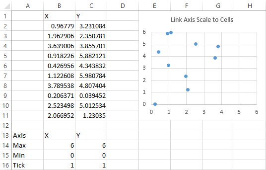
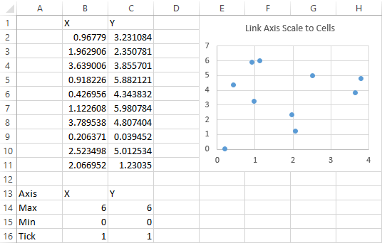 The cells B14:C16 can contain static values which the user can manually change, or they can contain formulas with your favorite axis scaling algorithms. See how to set up axis-scaling formulas in
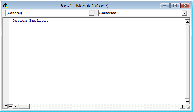
 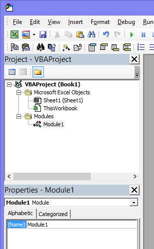 Double click on the module to open it. If there is no module, right click anywhere in the workbook’s project tree, choose Insert > Module. Or use Insert menu > Module. Up will pop a blank code module.
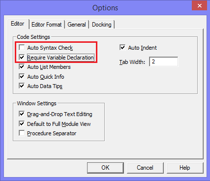
  If your module does not say Option Explicit at the top, type it in manually. Then go to Tools > Options, and in the Editor tab check the Require Variable Declaration checkbox. This will place Option Explicit at the top of every new module, saving innumerable problems caused by typos. While in the Options dialog, uncheck “Auto Syntax Check”. This will save innumerable warnings about errors you already know about because the editor turns the font of the offending code red.
  You can use a simple procedure that changes the axes on demand. The following changes the scales of the active chart’s axes using the values in B14:C16. Select the chart, then run the code.
 Select the chart and run the code. You can run the code by pressing Alt+F8 to open the Macros dialog, selecting the procedure in the list of macros, and clicking Run.
  Or you could
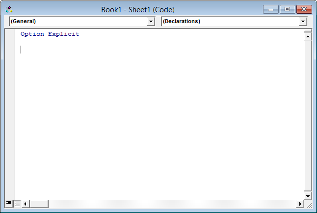 You can write the entire procedure yourself, but it’s easier and more reliable to let the VB Editor start it for you. Click on the left hand dropdown at the top of this module, and select Worksheet from the list of objects.
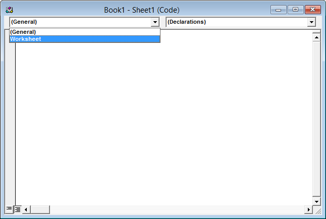 This places a stub for the Workbook_SelectionChange event in the module. Ignore this for now. Click on the right hand dropdown at the top of this module, and select Change from the list of events.
 You now have a couple event procedure stubs.
 Delete the Worksheet_SelectionChange stub, which we will not be needing, and type or paste the Worksheet_Change code into the Worksheet_Change stub.
 The code is given below, so you can copy it. When the event fires, it starts the procedure, passing in Target, which is the range that has changed. The procedure uses Select Case to determine which cell was changed, then changes the appropriate scale parameter of the appropriate axis.
