Lambda Moving Average Formulas

In two recent articles, Excel Lambda Moving Average and Improved Excel Lambda Moving Average, I described my efforts to build a Lambda moving average formula that worked the way I wanted it to. I’ve included average calculations for the first few data points before the number of points being averaged is met. I’ve also included only counting points within a set number of days, even if there are missing days within the range.

Here I will compare three different moving averages, the Simple Moving Average (SMA), the Weighted Moving Average (WMA), and the Exponential Moving Average (EMA), often called the Exponentially Weighted Moving Average (EWMA). I will develop Lambda functions for each, and I will show how to build up a data range that will enable a chart to update when the size of the range changes.

Moving Averages

Often data exhibits variation, and moving averages allow us to smooth out this variation. Our examples will apply seven-point moving averages to the following data set, consisting of 25 points that roughly follow a sine wave.

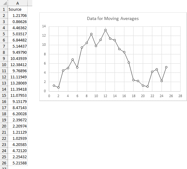
The downloadable workbook I used for this article is Lambda Moving Averages.xlsx.

Simple Moving Average (SMA)

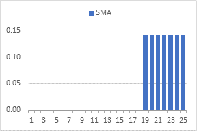
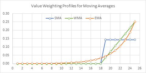
My previously cited efforts involved Simple Moving Averages. A Simple Moving Average simply averages a certain number of values to produce the averaged values. For our 7-point moving average, the contribution of each value to the last average is shown below. The last seven points equally contribute 1/7 of their value (0.142857…) to the average. Often at the beginning of the data range, when fewer values are available than the number to be averaged (7 in my example), no average is calculated. I prefer to modify the formula so it averages the available values.

Here is my Simple Moving Average Lambda formula from the recent article; the data to be averaged is located in A2:A26, and the number of points to average (7 for these examples) is in cell K1. These inputs are appended to the Lambda formula in parentheses.

=LAMBDA(arr, n,
  LET(
    sma, MAKEARRAY(
      ROWS(arr),
      1,
      LAMBDA(r, c,
        LET(
          movarr, TAKE(TAKE(arr, r), -n),
          AVERAGE(movarr)
        )
      )
    ),
    sma
  )
)(A2:A26, K1)

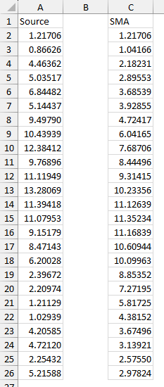
This formula is entered into cell C2, and here are the calculated Simple Moving Averages.

You can use the Advanced Formula Environment (or AFE instead of its full name which is rather long to cram into the ribbon) to edit the Lambda function.

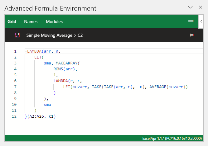
The AFE is easier to use than the built-in Formula Bar editor, it includes all of the usual IntelliSense, and it smartly adds line breaks and spaces to make the formula easier to read. Here is what the formula looks like in the AFE; Grid is selected in the second row indicating that the AFE is evaluating a cell formula. (Note: I do most of my editing in the old-school Formula Bar and in Notepad++, but I’m starting to transition to the AFE).

We can use that Lambda function, without the parenthetical arguments at the end, to define a Name that will serve as a function, as a User-Defined Function if you will; we can use this function anywhere in the workbook. On the Formulas tab of the ribbon, click on Define Name to pop up the New Name dialog.

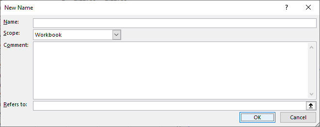
Enter a function name (in Name), a brief description (in Comment), and the formula (in Refers To).

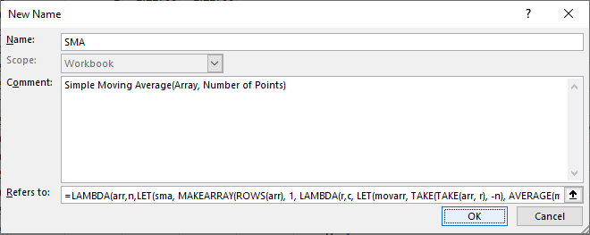
Click Enter, and the SMA function becomes available for use throughout the workbook.

This Name (John Walkenbach coined the phrase “Named Formula” decades ago) can also be added using the Advanced Formula Environment. and of course, the AFE can be used to edit any existing Named Formulas. Our SMA Named Formula is shown below in the AFE; Names is selected in the second row to indicate that the AFE is evaluating a Named Formula. Note that it does not show the outermost Lambda, and Formula Name and its Arguments are specified in their own sections of the dialog. This was confusing to me the first several times I tried using the AFE in this way, but I’m learning.

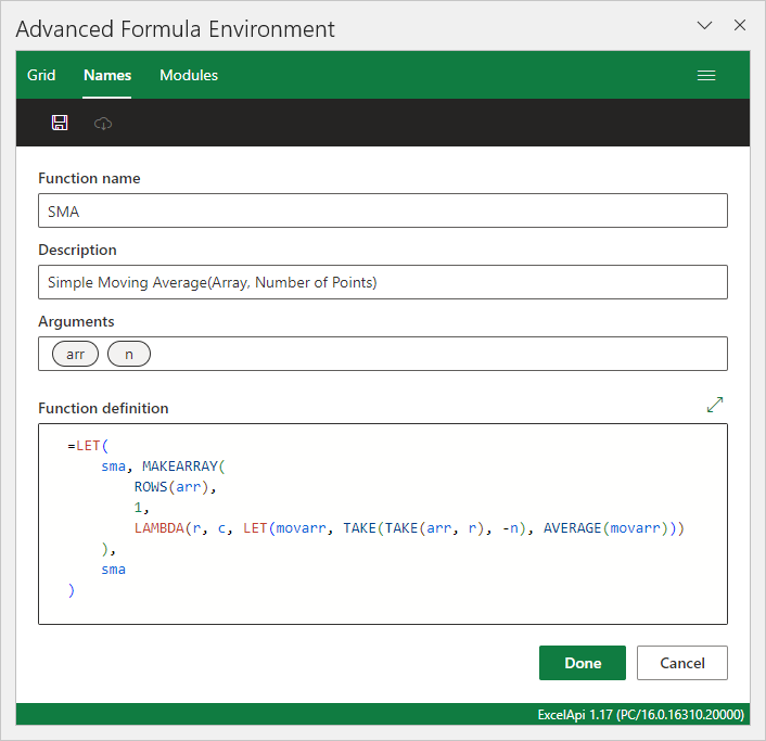
The function SMA can be used anywhere; it is used in cell E2 below as simply

=SMA(A2:A26,K1)

The results of this formula in E2 (spilling down to C26) match those of the Lambda function in cell C2.

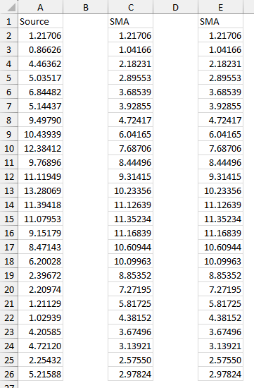
I usually create my Lambda formulas in a cell, as in cell C2 above, then copy and paste it into a Name, where it becomes a reusable user-defined function.

I promised a technique to make a chart recognize the dynamic nature of the Dynamic Arrays produced by these Lambda functions. Charts dynamically update when their data is contained in a Table, and the Table resizes; see Easy Dynamic Charts Using Lists or Tables. Microsoft has recently extended this dynamic behavior to Dynamic Arrays; it’s not as reliable (yet) but it makes dynamic charts work despite Dynamic Arrays not being compatible with Tables. The only catch is that, at least so far, all of the chart’s data has to reside in the same Dynamic Array.

So I want to build a Dynamic Array with column headers, X values (point numbers), and Y values (original data and moving average). The headers are a simple array, {"Point","Data","SMA"}. The point numbers are a simple SEQUENCE function, the data simply links to the source data, and SMA is calculated using our Lambda function. We can use HSTACK to stack the point numbers, data values, and moving averages, then use VSTACK to stack the headers on top of this HSTACKed block. Our formula is

=LAMBDA(array, num,
  LET(
    output, VSTACK(
      {
        "Point",
        "Data",
        "SMA"
      },
      HSTACK(
        SEQUENCE(
          ROWS(array)
        ),
        array,
        SMA(array, num)
      )
    ),
    output
  )
)(A2:A26, K1)

This formula is entered into cell G1, and it produces the range used to plot the data.

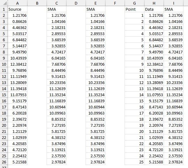
Here is our data plotted with the Simple Moving Average.

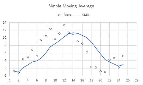
Most moving averages are based on historical data, so they lag behind the data. Therefore the Simple Moving Average is a trailing measure. It does not reach as high or low as the original data, and it changes direction later than the original data. But it is also smoother than the original data. The more points being averaged, the greater the lag and the smoother the curve.

Dynamic Charts from Dynamic Arrays

To illustrate how Dynamic Arrays can make a chart dynamic, let’s look at the following chart and DA source data. The top left cell uses the previous formula, but its final arguments are (A2:A15, K1), so it is only looking at 14 data points.

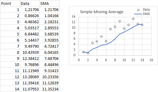
If all we do is change our arguments to (A2:A26, K1), the Dynamic Array expands to 25 points, and the chart automatically expands to include all 25 points. This behavior was astounding in Excel 2003 when its new Lists feature (renamed Tables in Excel 2007) allowed charts to react when their source data ranges expanded, and it is astounding in Excel 365 when combined with equally astounding Dynamic Arrays.

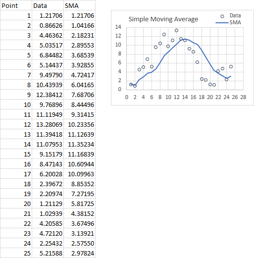
This link between a chart and a Dynamic Array is not as “smart” as the one between a chart and a Table. But if you are using an XY Scatter Chart, or if you are only making simple changes, like adding rows, the dynamics are amazing.

Weighted Moving Average (WMA)

A Weighted Moving Average applied different weights to the data values to produce the averages. In principle you could apply whatever weights you want, but for a moving average, often a triangular pattern is used, which gives more emphasis to the most recent values. These weights are the array {1, 2, 3, … 7}. The last value is multiplied by 7, the next to last by 6, all the way to the seventh from last by 1; these are added together and divided by the sum of the weights, which is 28. These normalized weights for our 7-point moving average, the contribution of each value to the last average calculated, is shown below.

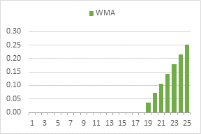
Here is my Weighted Moving Average Lambda formula; it is not much more complicated than the Simple Moving Average. As before, the data to be averaged, in A2:A26, and the number of points to average, in cell K1, are appended in parentheses to the Lambda formula.

=LAMBDA(arr, n,
  LET(
    wma, MAKEARRAY(
      ROWS(arr),
      1,
      LAMBDA(r, c,
        LET(
          movarr, TAKE(TAKE(arr, r), -n),
          m, ROWS(movarr),
          weight, SEQUENCE(m) * 2 / m / (m + 1),
          SUM(movarr * weight)
        )
      )
    ),
    wma
  )
)(A2:A26, K1)

I’ll go through the same progression as I did while developing the Simple Moving Average function above. If you get bored, feel free to scroll along at your own pace.

This formula is entered into cell C2, and here are the calculated Weighted Moving Averages.

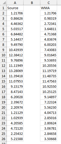
We can follow the same procedure as above, using the Define Names dialog or the Advanced Formula Environment to define a Named Formula called WMA. We can then call this formula using a simple formula.

=WMA(A2:A26,K1)

This formula is entered into cell E2 and displays the same calculations as the longer LAMBDA in C2.

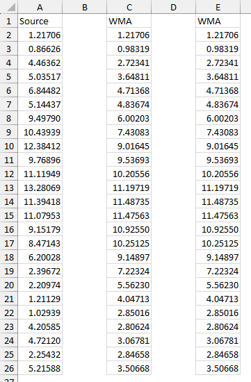
I didn’t need to duplicate the calculations, but I wanted to make sure they matched.

We can write another LAMBDA to stack together headers, point numbers, original data, and calculated Weighted Moving Averages.

=LAMBDA(array, num,
  LET(
    output, VSTACK(
      {
        "Point",
        "Data",
        "WMA"
      },
      HSTACK(
        SEQUENCE(
          ROWS(array)
        ),
        array,
        WMA(array, num)
      )
    ),
    output
  )
)(A2:A26, K1)

Here is the result when we enter this formula into cell G1; we can use this range to plot the data.

Again, the duplication isn’t strictly necessary, but it serves to validate the results. In fact, in my original workbook I had extra columns with conventional formulas to calculate my moving averages.

Here is the data plotted with the Weighted Moving Average.

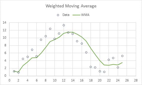
Like the Simple Moving Average, the Weighted Moving Average lags behind the original data while smoothing it. We’ll compare the various moving averages later.

Exponential Moving Average (EMA)

An Exponential Moving Average is calculated using this formula:

EMA_n = k * X_n + (1 – k) * EMA_n-1

where X_n is the current value, EMA_n is the current calculation, EMA_n-1 is the previous calculation, and k is the Exponential Smoothing Factor.

Note: The Exponential Moving Average (EMA) is sometimes referred to as the Exponentially Weighted Moving Average (EMWA).

The smoothing factor can be somewhat arbitrary, but when used in conjunction with N-point Simple or Weighted Moving Averages, it is often computed as

k = 2 / (N + 1)

For our example, k = 2 / (N + 1) = 2 / (7 + 1) = 2 / 8 = 0.25. This results in an effective weighting profile as shown below. The latest point is weighted the most, the previous point somewhat less, and earlier points increasingly less, but the weight never drops to zero.

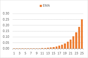
We can see that the weighting fits an exponential distribution if we plot the weights on a scatter plot and draw a trendline (below left); on a semilog plot (below right), the trendline is a straight line.

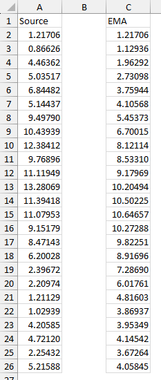
Our LAMBDA uses SCAN to calculate the Exponential Moving Average. The first value is the first element of the input array, and each subsequent calculation multiplies the previous value by (1 – k) and adds it to k times the current value.

=LAMBDA(arr, n,
  LET(
    k, 2 / (n + 1),
    ema, SCAN(
      INDEX(arr, 1),
      arr,
      LAMBDA(a, b, a * (1 - k) + b * k)
    ),
    ema
  )
)(A2:A26, K1)

I’m repeating the same progression as with the Simple and Weighted Moving Average functions above. Feel free to jump ahead.

Entered into Cell C2, this formula produces the following calculations.

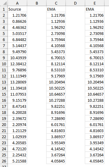
Let’s define another formula, EMA, to complete our family of Moving Average LAMBDAs. We call it like this:

=EMA(A2:A26,K1)

Entered into cell E2, we compute the moving averages as shown.

Again, we can build a LAMBDA to combine headers and columns of values into a single Dynamic Array.

=LAMBDA(array, num,
  LET(
    output, VSTACK(
      {
        "Point",
        "Data",
        "SMA",
        "WMA",
        "EMA"
      },
      HSTACK(
        SEQUENCE(
          ROWS(array)
        ),
        array,
        SMA(
          array,
          num
        ),
        WMA(
          array,
          num
        ),
        EMA(array, num)
      )
    ),
    output
  )
)(A2:A26, I1)

The Dynamic Array appears when this formula is entered into cell G1.

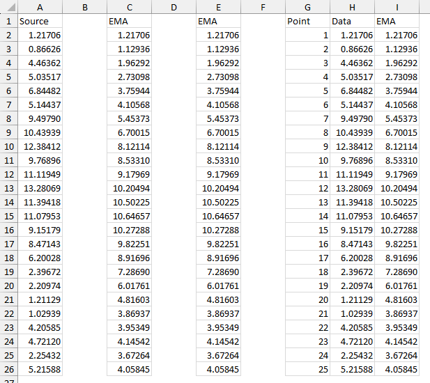
That data can be plotted, to show the the Exponential Moving Average behaves in a similar way to the others, trailing the actual data while smoothing it out.

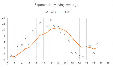
Like the Simple and Weighted Moving Averages, the Exponential Moving Average lags behind the original data.

Comparing the Moving Averages

Since we have already defined our Moving Average functions, we can write the following LAMBDA Dynamic Array formula to build a block of cells that we can use for a chart.

=LAMBDA(array, num,
  LET(
    output, VSTACK(
      {"Point", "Data", "SMA", "WMA", "EMA"},
      HSTACK(
        SEQUENCE(ROWS(array)),
        array,
        SMA(array, num),
        WMA(array, num),
        EMA(array, num)
      )
    ),
    output
  )
)(A2:A26, I1)

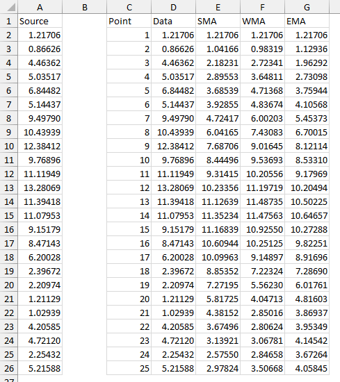
Entered into cell C1, the formula produces this data in the worksheet.

Here is that block of data plotted in an XY Scatter Chart.

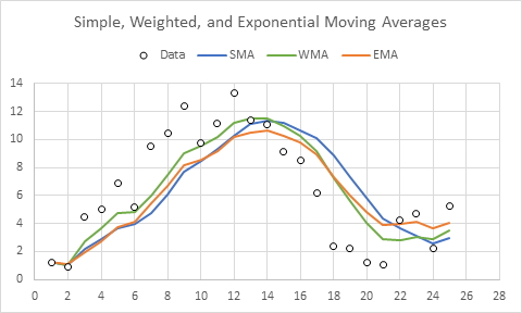
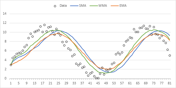
All three of the Moving Averages lag changes in the data. The Simple Moving Average lags more than the others, because the weights for the last few values are lower than for the other averages. The Weighted Moving Average follows the data most closely, because it only includes the last seven points in its calculations, not all points in a long tail like the Exponential Moving Average.

If we look at a different data set, again roughly a sine wave but including many more points, and average more points, we can compare the three Moving Averages in more detail.

Where the LAMBDA Functions Live

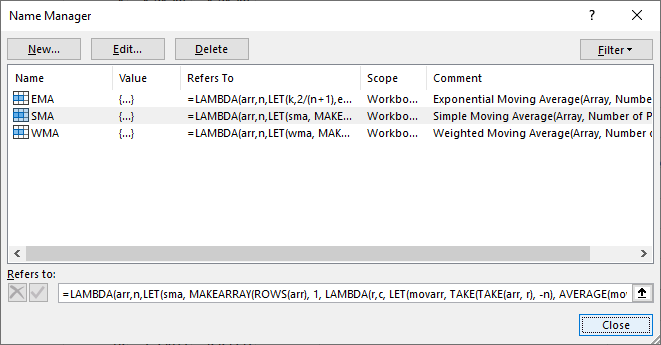
Our user-defined LAMBDA functions are saved in the workbook as Names, or Named Formulas. You can access them in the Name Manager on the Formulas tab of the ribbon (or using Ctrl+F3). The LAMBDAs are listed along with any other Names defined in the workbook. Select one to see a bit more of its definition in the Refers To box at the bottom (unfortunately it does not support line wrapping, right Microsoft?), and click the Edit button to see it in more detail (also not line-wrapped).

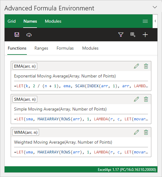
You can also use the Advanced Formula Editor, selecting names in the second row to view all of your Named LAMBDAs. Click on the pencil icon next to a LAMBDA to view it in more detail.

When you have created LAMBDA functions, they live in a specific workbook, and are not available in other workbooks. However, if you copy a worksheet from the workbook that has the LAMBDAs into a workbook without the LAMBDAs, your LAMBDAs go with the sheet into the second workbook. This is convenient, but also can cause confusion, as anyone knows if they have worked extensively with Names.

References

Moving Average, Weighted Moving Average, and Exponential Moving Average

How Is the Exponential Moving Average (EMA) Formula Calculated?

More Articles About Dynamic Arrays, LET, and LAMBDA

• ISPRIME Lambda Function
• Improved Excel Lambda Moving Average
• Excel Lambda Moving Average
• LAMBDA Function to Build Three-Tier Year-Quarter-Month Category Axis Labels
• Dynamic Array Histogram
• Calculate Nice Axis Scales with LET and LAMBDA
• VBA Test for New Excel Functions
• Dynamic Arrays, XLOOKUP, LET – New Excel Features