Dynamic Charts in Excel
Dynamic Charts with Names
In the oldest versions of Excel, the only way to make a chart dynamic was by defining Names for the chart’s X and Y values and using these Names in the chart’s SERIES formulas. (Names are also called Named Ranges and more accurately Named Formulas.) If a chart is plotted by column, adding rows will add points to the series in a chart, but adding columns will not add series to the chart; this points-only dynamic behavior is a weakness of these charts. Read my ancient tutorial about Dynamic Charts in Excel.
Dynamic Charts with Tables
More recently (starting over two decades ago), you could convert your data range to a Table (or in Excel 2003, a List) and a chart using all the data in that Table would dynamically change its data range to match the changing size of the Table. This is much easier than defining and applying all the required Names to the chart, and the chart adds both points and series as the Table grows in two directions. Read about Easy Dynamic Charts Using Lists or Tables.
Dynamic Charts with Dynamic Arrays
Soon after Microsoft introduced Dynamic Array formulas to Excel, they linked a chart’s source data range to a Dynamic Array’s spill range in a similar way. When a Dynamic Array’s spill range changes, a linked chart’s source data adjusts to keep up with the Dynamic Array, adding points and series as the spill range adds rows and columns. Microsoft first announced Dynamic array support in charts (Insiders Beta) in the September 2022 edition of What’s New in Excel. I’ve discussed this in Dynamic Charts Using Dynamic Arrays.
Dynamic Charts with Dynamic Arrays and Names
Despite the ease of using Dynamic Arrays to populate dynamic charts, you may wish to define Names based on the Dynamic Arrays, and build a dynamic chart with these Names.
One reason to define names for your dynamic charts is that Dynamic Array linkage to charts is not totally reliable. At the time of this writing, the chart data range is distorted if you insert or delete a row anywhere above the spill range or insert or delete a column to the left of the spill range.
Another reason is that if the Dynamic Array returns an error (e.g., #CALC!), the chart’s source data range may reset itself and not be restored when the error is fixed.
A third reason is that there may be several columns of Dynamic Arrays, with numerous charts that show only some of these columns. Naming the individual columnar ranges is the easiest way to make such charts dynamic.
I’ll walk through the process in this article. You can download the accompanying workbook here:
Dynamic Arrays, Names, and Charts.xlsx
Charting Static Data
This is the basis of my simple example. The data in cells B4:C8 has been plotted in an XY Scatter chart. I’ve color-coded the data in this article to correspond with the highlight colors seen in the worksheet when a chart is selected: red for series names, purple for X values, and blue for Y values. The SERIES formula for the single series in the chart is shown below the chart.
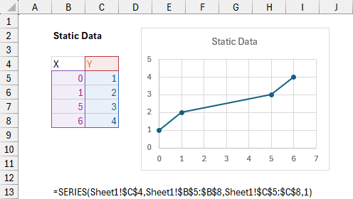
If the data range is extended by adding a row or column of data below or to the right of the data range, the static chart will not update.
Charting a Dynamic Array
Here I’ve created a Dynamic Array in B18:C22 by entering the formula =B4:C8 in cell B18. Most Dynamic Arrays you encounter will use much more elaborate formulas, and may change in size according to the various inputs. The color-coded range is plotted in the XY Scatter chart, and the SERIES formula is shown below the chart.
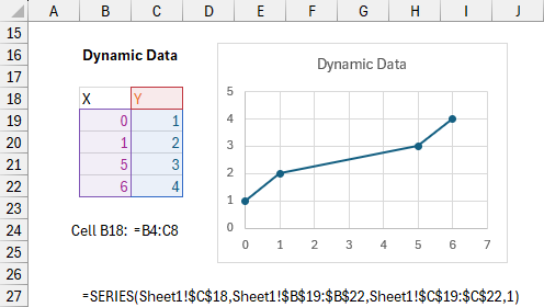
If the Dynamic Array were to change size, the chart source data would change accordingly, adding or removing points or series. I have not caused the spill range to change size, I leave that as an exercise to the reader.
Charting Names Based on Dynamic Arrays
I was going to use INDEX() formulas to define my Names, but my first attempt didn’t work. I switched to OFFSET() formulas, found a glaring user error, then fixed the INDEX() formulas. So I’ll show both OFFSET and INDEX versions. INDEX is preferred because OFFSET is volatile, while OFFSET formulas may be easier to construct from non-Dynamic-Array ranges. Again, I will not demonstrate the dynamic nature of Dynamic Array Name formulas
Using OFFSET Names
It’s helpful to construct and test formulas before using them in Names. In cell N5 I entered this formula:
=OFFSET(B18#,0,1,1,1)The hash nomenclature B18# means use the spill range of the formula in cell B18; this is shorthand in our example for B18:C22, but the bottom right address C22 is not hard-coded in the address. From this Dynamic Array spill range, I offset zero cells down and one cell right, and resize it to one row tall and one column wide.
I enter these formulas in cells L8 and N8:
=OFFSET(B18#,1,0,ROWS(B18#)-1,1)
=OFFSET(B18#,1,1,ROWS(B18#)-1,1)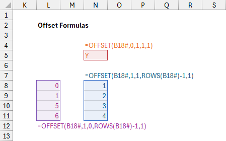
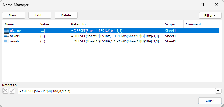
Each of these color-coded ranges match the corresponding parts of the Dynamic Array’s spill range, so I can use these formulas as the basis of my Names. The names and their Refers To definitions are shown below: the “o” prefix on the names stands for “OFFSET”. I’ve made minor changes to the Refers To formulas: I’ve used absolute references $B$18 rather than B18, so the formulas don’t change when the active cell move, and I’ve prefixed the cell address with the sheet name. I’ve also defined the Names with a scope of Sheet1.
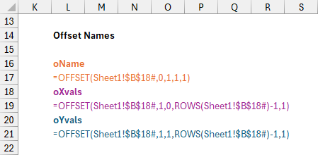
A quick refresher about creating a Name. Go to the Formulas tab, and click on Define Name. Give the Name a name (ugh, nomenclature!), assign a Scope of Sheet1, enter a comment if desired, and enter the Refers To formula, then click OK.
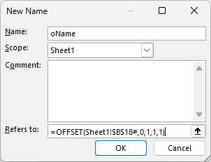
You can review the Names by pressing Ctrl+F3. The Name Manager lists the names, the Refers To formulas, and other details. Click in the Refers To formula box, and the defined range is highlighted in the worksheet.
If you often work with Names, the built-in Excel Name Manager is far surpassed by a free Name Manager developed by my colleague Jan Karel Pieterse.
To make sure that these Names work as intended, I scrolled down and entered
=oName
=oXvals
=oYvals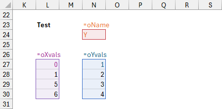
into cells N24, L27, and N27. These agree with the OFFSET formulas above and with the Dynamic Array, so they are safe to use in the chart.
Here is the dynamic chart based on Names built from our Dynamic Array. I copied my original chart and changed the SERIES formula from
=SERIES(Sheet1!$C$4,Sheet1!$B$5:$B$8,Sheet1!$C$5:$C$8,1)to
=SERIES(Sheet1!oName,Sheet1!oXvals,Sheet1!oYvals,1)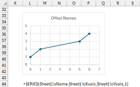
This chart will add points as the Dynamic Array adds rows, though adding columns will not add series to the chart.
Using INDEX names
I started building my INDEX Names by entering this formula in cell W5:
=INDEX(B18#,1,2)From this Dynamic Array spill range B18#, I selected the cell in the first row and second column.
I enter these formulas in cells U8 and W8, which basically mean drop the first cell (the header) from the first and second columns of the spill range:
=DROP(INDEX(B18#,0,1),1)
=DROP(INDEX(B18#,0,2),1)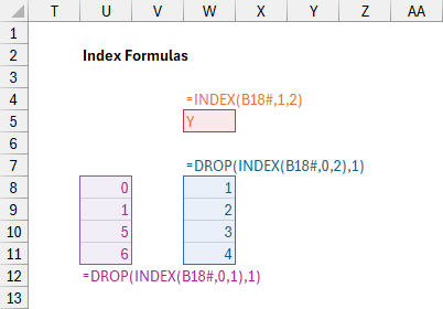
These color-coded ranges match the corresponding parts of the Dynamic Array’s spill range, so I will use these formulas as the basis of my Names. The names and their Refers To definitions are shown below: the “i” prefix on the names stands for “INDEX”. I changed the relative reference B18 to absolute reference $B$18, which caused the error in my first attempt, and I’ve prefixed the cell address with the sheet name. I’ve defined the Names using Sheet1 as the scope of the Name.
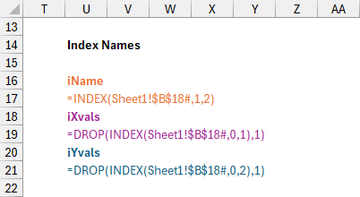
To make sure that these Names work as intended, I scrolled down and entered
=iName
=iXvals
=iYvals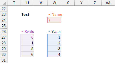
into cells W24, U27, and W27. These agree with the INDEX formulas above and with the Dynamic Array, so I can use them in the chart.
Here is the dynamic chart based on Names built from our Dynamic Array. I copied my original chart and changed the SERIES formula from
=SERIES(Sheet1!$C$4,Sheet1!$B$5:$B$8,Sheet1!$C$5:$C$8,1)to
=SERIES(Sheet1!iName,Sheet1!iXvals,Sheet1!iYvals,1)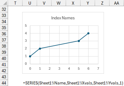
This chart is dynamic, adding points as the Dynamic Array adds rows, but adding columns will not add series to the chart.
Dynamic Array Chart Articles
- Dynamic Charts Using Dynamic Arrays
- Dynamic Array Histogram
- LAMBDA Function to Build Three-Tier Year-Quarter-Month Category Axis Labels
Dynamic Chart Articles
- Dynamic Charts
- Easy Dynamic Charts Using Lists or Tables
- Dynamic Charts in Excel 2016 for Mac
- Dynamic Chart using Pivot Table and Range Names
- Dynamic Chart using Pivot Table and VBA
- Dynamic Ranges to Find and Plot Desired Columns
- Split Data Range into Multiple Chart Series without VBA
- VBA to Split Data Range into Multiple Chart Series
- Dynamic Chart Source Data (VBA)
- Dynamic Chart with Multiple Series
- Display One Chart Dynamically and Interactively


Leave a Reply