In Graphical Approach to a Simple Physics Problem I discussed my daughter’s physics homework. The problem was to determine the relationships between how long it takes water to drain from a hole in the bottom of a bucket, the diameter of this hole, and the initial height of water in the bucket. The data is shown in this table.

The first step is to plot the data using XY charts. The charts below show time to drain vs height for various hole sizes and time to drain vs hole size for various diameters. We will investigate various trendline formulas using these plots.
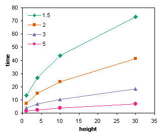
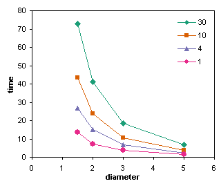
In Trendline Fitting Errors I warned about picking an appropriate type of trendline relationship. In Graphical Approach to a Simple Physics Problem I automatically looked for a power law relationship. What if I didn’t have a scientific background? How might I go about fitting trendlines to the data. Let’s just look at the highest curve in each of the charts above, and apply a few trendlines.
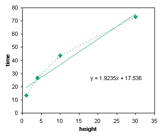
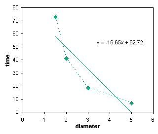
Obviously the lines are not linear, but let’s start with linear trendlines. The original data are shown with points connected by dotted lines, and the trendlines by solid lines.
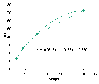
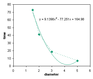
Since there is curvature in the data, we need a higher power of the X variable. These two charts show polynomial fits of order 2. The fits come close to fitting all of the points, but the curve for height seems to be approaching a maximum at a height of 30, implying that if we double the height, the time will decrease. The curve for diameter is even stranger, with a minimum just above 4; this implies that if we widen the hole further, the water will leak out more slowly. Both of these scenarios are rather unlikely.
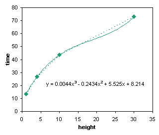
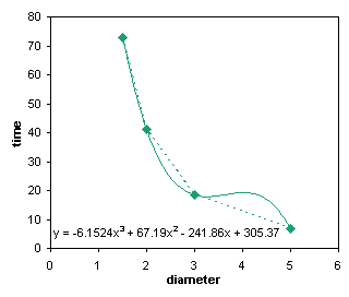
To carry the polynomial fitting to an extreme, let’s look at third order fits. Fortunately, with only four points, we will not be able to go beyond this. In the height relationship, the poly fit predicts a slowing of the increase of time with height, then after about 20 it accelerates. The diameter relationship actually changes direction twice. To smooth this out, we’d have to make another measurement at a height of 20 or a diameter of 4, then apply a higher order fit.
This turns into an exercise of reductio ad absurdum, and fortunately Excel doesn’t get more absurd than a polynomial fit of order 6. In my previous life as a scientist/engineer, there were very few physical relationships that theoretically followed polynomial relationships. Sometimes a poly fit was acceptable when interpolated values were required, but it’s generally better to find a simpler relationship. A simpler relationship is one with fewer fitting parameters, and which follows the form of any theoretical description of the phenomenon.
A great many physical phenomena follow power law relationships. The following show power law fits to the data.
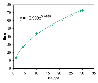
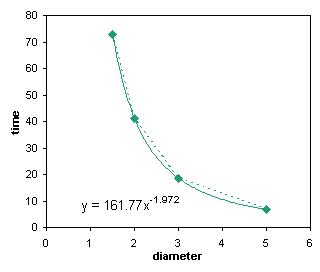
Time to drain the bucket follows the reciprocal of diameter to the second power. This fits nicely since the volume of water passing through the hole is proportional to the area of the hole, which is proportional to the diameter squared. It’s an inverse relationship, because the larger the hole, the more water can flow, and the shorter time it will take.
I’m less certain of the height relationship. The time is obviously additive as more water is added to the initial height. Also, the added water should push harder on the water beneath, forcing it out faster. An equal increment of water height will produce a decreasing increment of time. If I weren’t too lazy to dig my old calculus book out of the basement, I’d find the similar example and determine the exact form of the drainage curve.
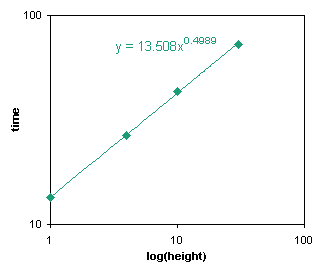
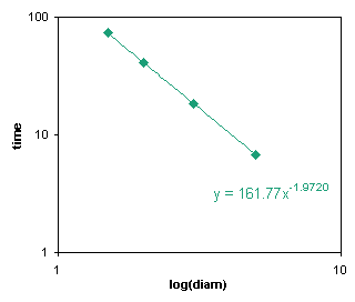
Below is another view of the power law fits on a double logarithmic scale (on which a power law fit traces a straight line). The visual goodness of fit lets me assert that the power law fits are appropriate.
More Trendline and Regression Articles on this Blog
- Trendlines and Chart Types in Excel
- Add One Trendline for Multiple Series
- Trendline Calculator for Multiple Series
- Trendline Fitting Errors
- Plot Two Time Series and Trendlines with Different Dates
- Polynomial Fit vs. Statistical Process Control
- Moving Averages
- Stacked Column Chart with Stacked Trendlines
- Deming Regression
- Deming Regression Utility
- LOESS Smoothing in Excel
- LOESS Utility for Excel


Michael says
Hi Jon –
Looking at the results, I want to jump to
y = 13.508x^.5 and y = 161.77x^-2
Lots of things in nature are squared relationships.
…mrt
Jon Peltier says
Michael –
“Lots of things in nature are squared relationships.”
Very true. One major problem with polynomial fits is that using them effectively separates the data from any resemblance to a physical model. I touched on this in Graphical Approach to a Simple Physics Problem, pointing out that the relationship to hole diameter squared was probably a linear first order relationship to hole area.
In follow-up discussions I will assume powers of 2 and 0.5 and show how to optimize the pre-exponential coefficient.
Jon2 says
Hi, great article and just what I was looking for.
I have a data set for a series of physical tests. The test is looking at the length of cuts which a blade makes in a material when the force applied to the blade is varied.
For something like this, could you comment on whether a power or an exponential trendline is more likely to be the correct way to go?
In my current data set there is very little difference between them, but that won’t necessarily be the case in future trials so I would welcome your advice.
Thanks in advance, and please note the link in the 3rd paragraph of the article to Trendline Fitting Errors returns error 404 :-)
Jon Peltier says
Jon2 –
It seems everyone likes power law relationships for physical processes. If you’re trying to understand the underlying mechanisms of the phenomenon under study, so many things are well-described by power laws. Of course, there are often little corrections, for example:
Y = k X^n becomes something like Y = Yo + k (X – Xo)^n
Of course, exponential relationships are not uncommon, but for a mechanics of materials kind of problem like this, I’d expect the power law to do a good job.