Chart Series Data Highlighting

In Chart Source Data Highlighting I described the highlighting that displays the source data range of a chart and enables adjustment of this range without entering dialogs and editing the series formula. When the chart is embedded in the same sheet that contains its data, the data range is highlighted with up to three rectangular outlines, when a series in the chart has been selected. The series formula appears in the formula bar.

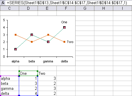
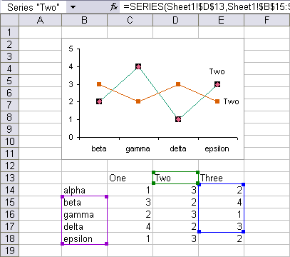
The X values are highlighted with a purple border, the series names with a green border, and the Y values with a blue border. If any of these parameters have not been defined, or they are not defined by a range in the chart’s parent worksheet, the corresponding colored borders are not displayed.

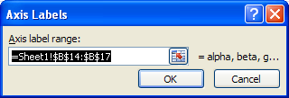
When the Source Data dialog (Excel 2003 and earlier) is displayed, the Series tab selected, and a series is picked in the Series list, the three ranges defining the series are shown in the various input boxes.

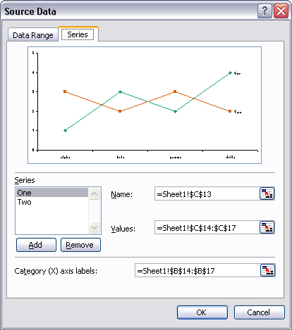
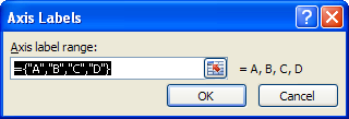
In Excel 2007 the series can be selected, but only the X axis values or labels can be seen, and there are no range references shown.

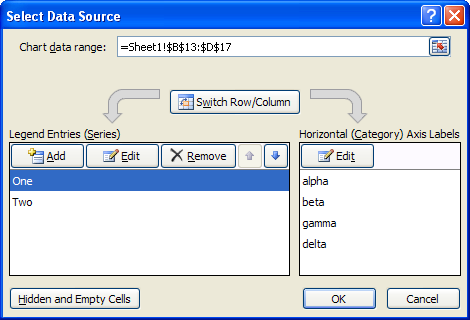
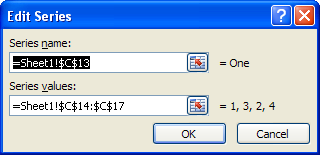
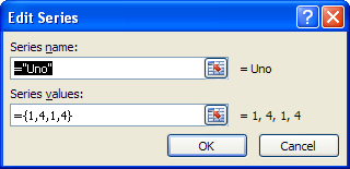
In one of Excel 2007’s most egregious insults to productivity, two child dialogs must be shown in sequence to see the ranges containing the series data ranges. It may be necessary to cycle back and forth several times before finishing with this dialog’s multiple windows.

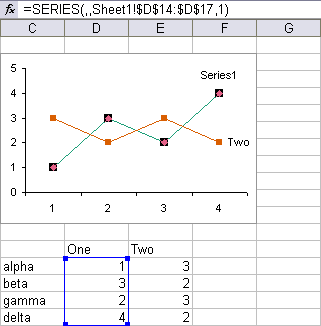
Only the arguments of the series formula that are defined in the sheet can be highlighted. In this chart, but o, series One has no name definend at all, only a blank slot in the series formula, so Excel applies the default “SeriesX” name. Likewise no X values have been specified, so Excel applies the counting numbers {1, 2, 3, etc.}. Only the Y values are higlighted in the worksheet.

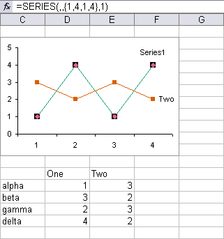
In this chart, not even the Y values can be highlighted, as they are defined by a hard-coded array.

All of this chart’s series One arguments are hard-coded: arrays for X and Y values and a text label for its name.

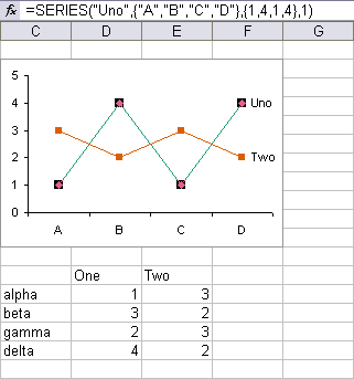
In the Source Data dialog, these parameters are indicated by text and arrays.

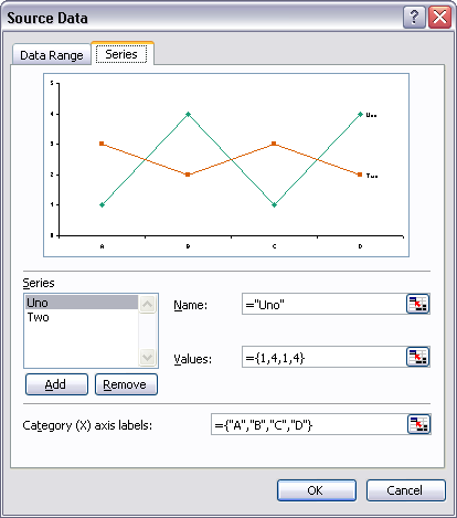
The same goes for Excel 2007

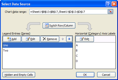
except of course that we have to dive twice into deeper layers of dialogs.

When a chart’s entire data range is highlighted, and the data for a series is moved independent of data for the other series, the highlighting breaks down. As long as each of the ranges remains contiguous, the data ranges for a series can still be displayed. In this example, it doesn’t matter that the Y values for series Two has been misaligned from its X values and series name.

This article provides a cleaner explanation of this topic, which was previously covered in Highlighted Chart Source Data.