Moving Averages
When averaging time-series data, you often want to smooth out peaks and valleys. A moving average is an easy way to smooth your data. When I track my weight, for example, I use a 7-day moving average. This smooths out peaks associated with weekends when I might go out to eat and enjoy a beer or two.
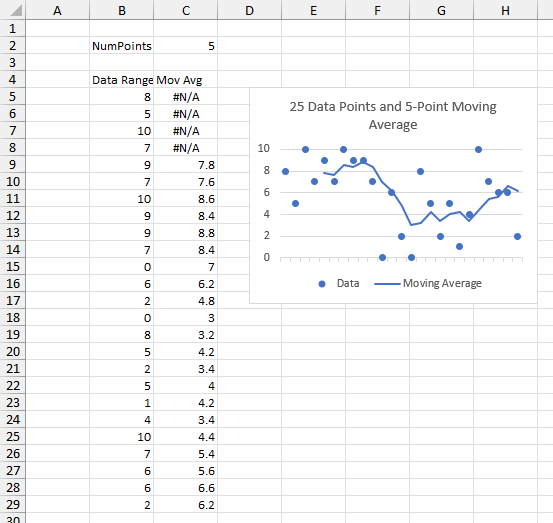
The image below shows 25 random data points and a five-point moving average. The points were generated with this Dynamic Array formula in cell B5:
=RANDARRAY(25,,0,10,TRUE)
and the moving average was calculated with this formula in cell C5, filled down to C29:
=IF(
  COUNT(OFFSET($B5,0,0,-$C$2,1))=$C$2,
  AVERAGE(OFFSET($B5,0,0,-$C$2,1)),
  NA()
)
When building large, complicated LAMBDA formulas, it has become common to enhance the readability of the formulas with line feeds (use Alt+Enter to insert a line feed in the Formula Bar) and spaces. I find it helps with older formulas as well.
This moving average formula needs to be placed in each row of the moving average range. If it’s in a Table, that’s no big deal, because adding more data will automatically fill the formula into added Table rows.
But the data was the result of a Dynamic Array formula in just cell B5, and the output spilled down as far as the formula required. It would be nice to build a Dynamic Array formula for moving average which is written just in cell C5 but spills down as far as the Dynamic Array it averages.
There are many formulas you can use to calculate a moving average, using variations of INDEX and OFFSET formulas. Incidentally, if you don’t need the moving average values in the worksheet, you can use an Excel chart’s trendline feature to display the moving average.
Internet Search for Dynamic Array Moving Average
I tried my hand at writing my own formula and got stuck almost immediately. I searched Bingle to see what I could find.
I found a lot of possible answers. The ones that seemed easy didn’t work. The ones that worked were very complicated, and I really didn’t understand them very well. I finally settled on one from Lambda Moving Average – calculate rolling sum in Excel (and much more). The original version of this function included a parameter that lets you choose whether to calculate a moving average or other moving statistical functions. I cleaned out all the other functions and was left with the moving average below:
=LAMBDA(x,window,
  LET(
    _x, x,
    _w, window,
    _thk, LAMBDA(x, LAMBDA(x)),
    _fn, _thk(LAMBDA(x, AVERAGE(x))),
    _i, SEQUENCE(ROWS(x)),
    _s, SCAN(
      0,
      _i,
      LAMBDA(a, b, IF(b < _w, NA(), _thk(MAKEARRAY(_w, 1, LAMBDA(r, c, INDEX(_x, b - _w + r))))))
    ),
    _out, SCAN(0, _i, LAMBDA(a, b, _fn()(INDEX(_s, b, 1)()))),
    _out
  )
)
As I said, it works fine, but I don’t really understand how it works. I’m reluctant to include it in a project for a client if I don’t grok it, but I’ve implemented it in some of my own workbooks. It seems to run slowly, probably because for each element of the original array, it generates a subset of that array to calculate an average. For an array with hundreds of points, that adds up to hundreds of smaller arrays.
I also went to ChatGPT to see what it could tell me. It showed me lots of code samples and several formulas that resembled Excel formulas. But many formulas had errors, and no formula that had no errors returned a moving average.
Running Sums?
I couldn’t wrap my tired, old brain around the algorithm above, but sometimes my brain gets bored, looks out the window, and surprises me with what it comes up with. And my approach isn’t rocket science, but it is less cumbersome than creating multitudes of arrays which all include partial duplicates of the original array’s values. I can calculate the running sum of the original array, subtract the running sum from an earlier row, and divide by the number of points, and I’ll have my moving averages.
First, I’ll show how it works. Here’s my data in the second column below. For reference I’ve inserted a sequence number in the first column. The gold-shaded range in the third column contains the running sum of the data in the second column. The fourth column contains the same shaded running sum, offset by 5 rows so I can compute my 5-point moving average. The first four cells of a 5-point moving average are not calculated; I’ve entered #N/A so they are not plotted.
Delta is the difference between the two running sums, that is, the intermediate moving sum, and Average is Delta divided by 5.
The first 5-point average is calculated for the 5th value, where the running sum is 39: 39 divided by 5 is 7.8.
The second calculation is for the 6th point, where the running sum is 46. But we only want the sum of points 2 through 6, so we subtract the running sum for point 1, which is 8. (46-8)/5 is 7.6. And so on.

Now let’s get it into a single formula.
Building the Formula
The following range illustrates the steps toward building the formula; several steps are just me learning how some new Excel functions work. Column B contains the original formula, and column C is my old-style formula-in-every-cell to calculate the moving average. I’ve hidden columns D:I.
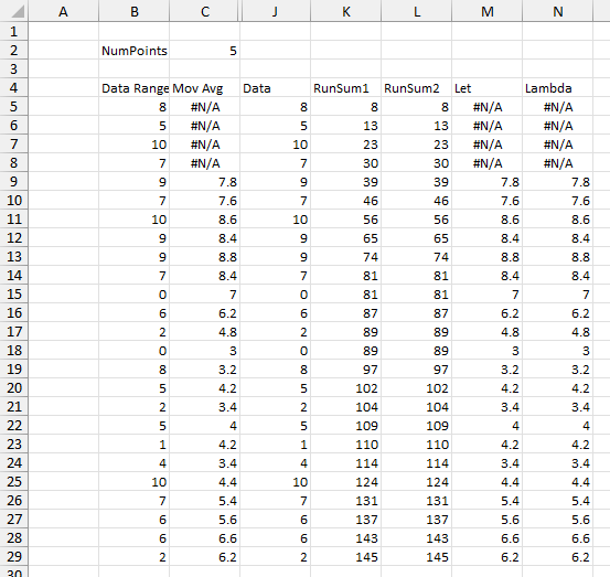
Column J spits out the original data range. This isn’t necessary in the final formula, but I was gaining confidence with BYROW. BYROW works by defining an array, passing it row by row into a LAMBDA function, and building an array of the results of that LAMBDA for each row. The array passed in is a simple SEQUENCE, from 1 to the number of rows in the original data range. Each element of the sequence is passed as x into LAMBDA, which returns the xth element of the data range.
=LET(
  datarange,B5#,
  BYROW(
    SEQUENCE(ROWS(datarange)),
    LAMBDA(x,INDEX(datarange,x))
  )
)
The running sum in column K is easy to calculate with the new Dynamic Array helper functions. Like BYROW, SCAN passes each element of an array into a LAMBDA function, which calculates each element of the output array, Again, this isn’t strictly necessary, but I was learning about SCAN.
The first argument of SCAN is the starting value (zero since it’s missing), the second is the original data range. LAMBDA accepts the starting value a and the data value b then applies the function a+b to generate the output value. This output becomes the new starting value a, which is added to the next data value b, etc.
=LET(
  datarange,B5#,
  SCAN(,datarange,LAMBDA(a,b,a+b))
)
The running sum in column L is a bit more convoluted, but it’s leading to my ultimate formula. SCAN is used as above to generate the running sum, but instead of spitting it out into the worksheet, it is stored in the name runsum. Then BYROW is used to return each element of runsum.
=LET(
  datarange,$B$5#,
  runsum,SCAN(,datarange,LAMBDA(a,b,a+b)),
  BYROW(
    SEQUENCE(ROWS(datarange)),
    LAMBDA(x,INDEX(runsum,x))
  )
)
If I can get the xth element of runsum, I can also get the element numpoints before that and subtract it. If x is less than numpoints, this corresponds to an early point which displays #N/A. If x is equal to numpoints, it’s the first calculated value, and there is no running sum to subtract, so I subtract zero. After subtracting to get the intermediate sum, I divide by numpoints to get the average.
=LET(
  datarange,$B$5#,
  numpoints,$C$2,
  runsum,SCAN(,datarange,LAMBDA(a,b,a+b)),
  BYROW(
    SEQUENCE(ROWS(datarange)),
    LAMBDA(x,
    IF(
      x<numpoints,
      NA(),
      (INDEX(runsum,x)-IF(x=numpoints,0,INDEX(runsum,x-numpoints)))
      /numpoints)
    )
  )
)
I can rewrite this as a LAMBDA:
=LAMBDA(datarange,numpoints,
  LET(
    runsum,SCAN(,datarange,LAMBDA(a,b,a+b)),
    BYROW(
      SEQUENCE(ROWS(datarange)),
      LAMBDA(x,
      IF(
        x<numpoints,
        NA(),
        (INDEX(runsum,x)-IF(x=numpoints,0,INDEX(runsum,x-numpoints)))
        /numpoints)
      )
    )
  )
)($B$5#,$C$2)
Note that the LAMBDA formula above ends with ($B$5#,$C$2), which is how these arguments are entered into the formula. To make this a reusable function, copy the formula without these arguments and their parentheses. Go to Formulas tab > Define Name. Enter a function name and short description, paste the formula into the Refers To box, and press Enter.
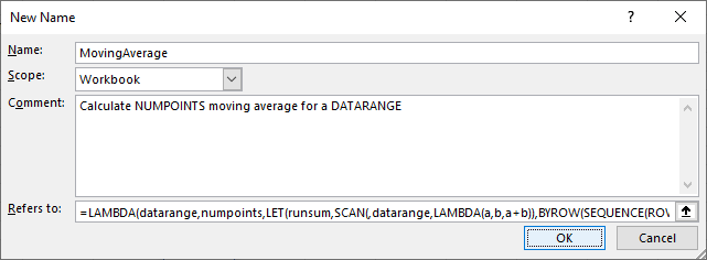
Using the Define Name method is suboptimal. The entire LAMBDA function cannot be viewed at once, and you lose the line feeds and white space. You could also use the Advanced Formula Environment, a free add-in from Microsoft.
You can now use this formula throughout the workbook using this simple syntax:
=MovingAverage(B5#,C2)
Improvements
I exchanged several comments on my earlier post with a smart reader named Henk-Jan van Well, who suggested several improvements to the moving average algorithm, starting with CHOOSEROWS, then evolving to TAKE and DROP. This led to simplified and more robust formulas, and also to a moving average by date which dealt nicely with missing dates, i.e., it averaged values within seven days rather than averaging seven consecutive values that may span more than seven days. See the improved post at Improved Excel Lambda Moving Average.
More About Dynamic Arrays, LET, and LAMBDA
- ISPRIME Lambda Function
- Lambda Moving Average Formulas
- Improved Excel Lambda Moving Average
- LAMBDA Function to Build Three-Tier Year-Quarter-Month Category Axis Labels
- Dynamic Array Histogram
- Calculate Nice Axis Scales with LET and LAMBDA
- VBA Test for New Excel Functions
- Dynamic Arrays, XLOOKUP, LET – New Excel Features


