In Grouping by Date in a Pivot Table I showed how to summarize daily data in a pivot table by grouping into monthly values. I’ll review this technique, then show how to clean up the dates when you don’t use the default starting and ending dates in the Grouping dialog.
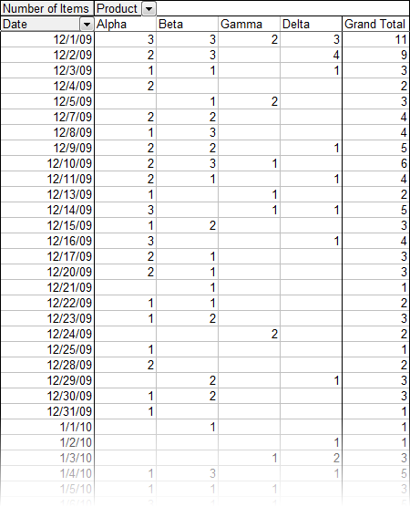
Here is a pivot table with daily values. I worked this out in Excel 2003, because that’s what was open at the time, but the technique is much the same in all versions. I want to condense this into monthly values, and show only data from 2010 and 2011.
I navigate to the Group and Show Detail > Group command, and choose the appropriate parameters in the Grouping dialog.
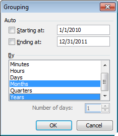
I change the range of dates in the pivot table by unchecking the two Auto boxes at the top and entering the start and finish dates I want. Then I select the time units I want the data grouped by. Pick Months and Years, or you’ll only get 12 monthly values summed over all the years within selected the date range.
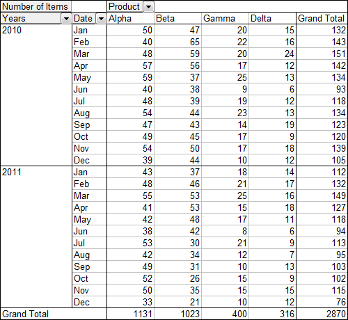
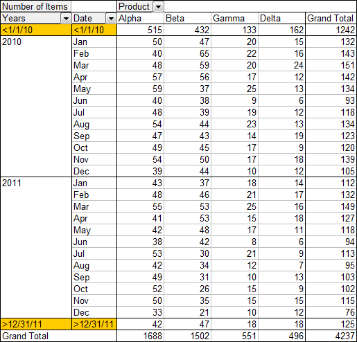
The pivot table is condensed into the desired time periods. The only problem is that Excel includes two additional pivot items in each date-related pivot field. The pivot fields Years and Date have pivot items <1/1/10 and >12/31/11 to account for data from outside our selected date range.
We can click on the field header dropdowns and see the pivot items in each. The Years and Date pivot item lists are shown below.
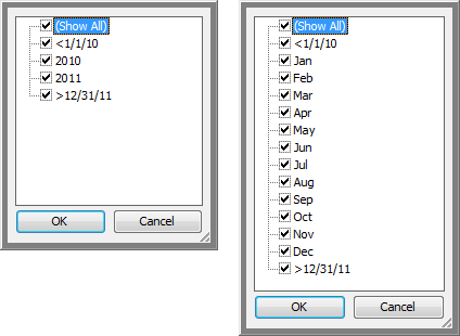
The pivot items have checkboxes, so we can manually uncheck the extraneous items, every time the pivot table is refreshed. Bo-o-o-oring.
I’ve actually been doing this manually for years in some of my accounting workbooks. Like the plumber’s faucet that always drips, the programmer’s workbook gets updated by hand. But a reader emailed me and asked how to get rid of those extra date items. I thought for about 30 seconds, and coded for about 3 minutes, and came up with this routine that cleans up any fields in the Row and Column areas of all pivot tables on the active sheet that have items beginning with “<” or “>”.
Sub Remove_GT_LT_PivotItems()
  Dim pt As PivotTable
  Dim pf As PivotField
  Dim pi As PivotItem

  For Each pt In ActiveSheet.PivotTables

    For Each pf In pt.RowFields
      For Each pi In pf.PivotItems
        If Left$(pi.Caption, 1) = "<" Or Left$(pi.Caption, 1) = ">" Then
          pi.Visible = False
        End If
      Next
    Next

    For Each pf In pt.ColumnFields
      For Each pi In pf.PivotItems
        If Left$(pi.Caption, 1) = "<" Or Left$(pi.Caption, 1) = ">" Then
          pi.Visible = False
        End If
      Next
    Next

  Next

End Sub
Here is the finished pivot table.
