Dynamic Chart Using Defined Name for Source Data
A dynamic chart can be constructed using dynamic ranges that change in size as data is added or removed. This technique is very powerful: you can define flexible ranges limited only by your ability to write an appropriate Refers To formula.
One limitation of this approach is that it can only account for dynamic numbers of points in a series, but not dynamic numbers of series in a chart. Using VBA you can work around this limitation.
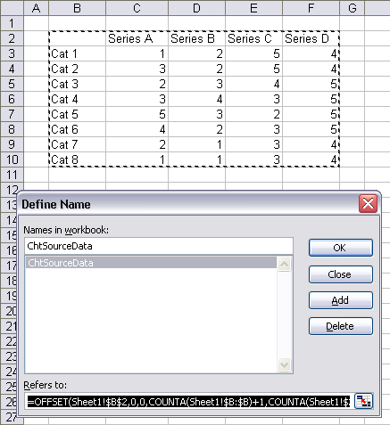
Let’s start with a simple data range as shown below. Following best practices, the data is arranged with series in columns, the category labels (X values) are in the first column, the series names are in the first row, and the top left cell of the range is blank. Using the Define Names dialog, we can define a name using these parameters:
Name: ChtSourceData
Refers To: =OFFSET(Sheet1!$B$2,0,0,COUNTA(Sheet1!$B:$B)+1,COUNTA(Sheet1!$2:$2)+1)
When we click Add and then click in the Refers To box, the range defined by the Refers To formula is highlighted by the marching ants border.

When creating a chart, or editing its source data, we can enter a dynamic range name in the Data Range box.
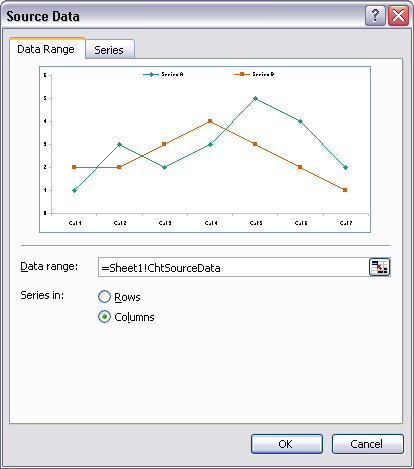
Excel accepts this definition of the chart data, but it converts the dynamic range name to a static range address. This means that our chart does not update as the dynamic range changes in size.

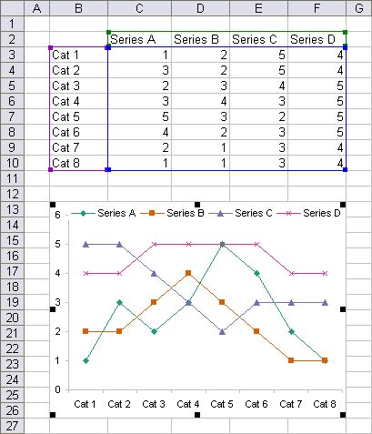
Here is our chart created with the dynamic range ChtSourceData. When the plot area or chart area of the chart is selected, the source data is highlighted.

Add some data to enlarge the dynamic range. Open the Define Names dialog, select ChtSourceData, and click in the Refers To box: The highlighted range shows that the dynamic range has enlarged to include all the added data.
The chart has not changed, but with a simple VBA procedure we can change the chart’s source data range to reflect the new dimensions of our defined range:
Sub UpdateChartSourceData()
  With ActiveSheet
    .ChartObjects(1).Chart.SetSourceData _
        Source:=.Range("ChtSourceData"), _
        PlotBy:=xlColumns
  End With
End Sub
This procedure should be placed into a regular code module, as described in How To Use Someone Else’s Macro.
Here is the updated chart:
To make this work more dynamically, you can include the SetSourceData command in a Worksheet_Change event. Right click on the sheet tab, choose View Code, and the VB Editor will appear with a code module representing the active sheet. Put this procedure into the module:
Private Sub Worksheet_Change(ByVal Target As Range)
  If Not Intersect(Target, Me.Range("ChtSourceData")) Is Nothing Then
    Me.ChartObjects(1).Chart.SetSourceData _
        Source:=Me.Range("ChtSourceData"), _
        PlotBy:=xlColumns
  End If
End Sub
This procedure executes whenever there is a change to a cell on the worksheet (not a calculation, but a change in an entered value or formula). The If checks whether the change occurred within the dynamic range ChtSourceData; if so, it resets the chart’s source data range. It’s automagic.
Better Way: Dynamic Chart Using Table for Source Data
There’s an easier way to make your whole chart dynamic, adding or removing points or series in the chart as rows and columns are removed or added in the source data range. This approach uses an Excel Table; it does not require brain bending Name definitions, and it doesn’t require any VBA coding. All it requires is that the chart uses a simple contiguous rectangular range.
The first step is to select the data range, and press Ctrl+T. A dialog pops up: make sure the indicated range is correct, and the Excel guesses correctly about headers, and click OK.

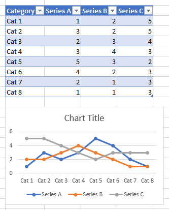
The range is formatted as a Table, and has the tell-tale filter dropdown buttons in the top row.

Since the chart uses the entire table for its data, meaning X and Y values use all columns of the table, series names use the header row of the table, and the series points use all rows, then if the size of the table changes by adding or removing rows or columns, the chart will continue to use the entire table, and will add or remove series and points to the chart.
This is just one example of the power and flexibility of Excel’s Tables.


