The Excel Chart SERIES Formula

Data in an Excel chart is governed by the SERIES formula. This formula is only valid in a chart, not in any worksheet cell, but it can be edited just like any other Excel formula.

The SERIES Formula

Select a series in a chart. The source data for that series, if it comes from the same worksheet, is highlighted in the worksheet. And a formula appears in the Formula Bar.

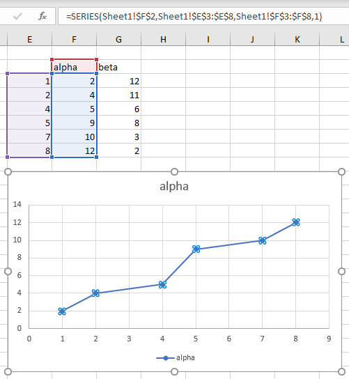
You didn’t have to write the formula. Excel writes it for you when you create a chart or added a series.

The formula in the chart shown above is:

=SERIES(Sheet1!$F$2,Sheet1!$E$3:$E$8,Sheet1!$F$3:$F$8,1)

The arguments are identified as follows:

=SERIES(<series name>,<x values>,<y values>,<plot order>)

In the case of a bubble chart, there is one additional argument:

=SERIES(<series name>,<x values>,<y values>,<plot order>,<bubble size>)

You can also view the series data using the Select Data dialog. Right click on the chart and choose Select Data, then select the series in the list and click the Edit button. The Edit Series dialog shows the same data that the SERIES formula shows.

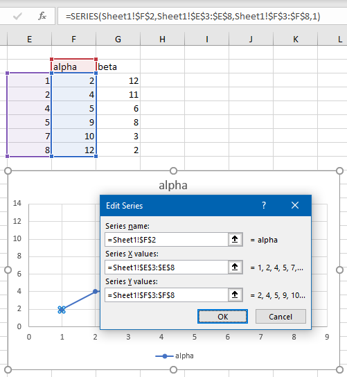
Here are a few valid SERIES formulas. This formula has conventional cell addresses:

=SERIES(Sheet1!$F$2,Sheet1!$E$3:$E$8,Sheet1!$F$3:$F$8,1)

This formula plots the same, although the values are not linked to the worksheet, but are instead hard-coded into the formula:

=SERIES("alpha",{1,2,4,5,7,8},{2,4,5,9,10,12},1)

This formula doesn’t even include a Series Name or Y Values, and the Y Values are represented by a Name (Named Range).

=SERIES(,,SERIESFormula!YValues,1)

Series Formula Arguments

Series Name

Series Name is obviously the name of the series, and it’s what is displayed in a legend. This argument is usually a cell reference, Sheet1!$F$2, but it can also be a hard-coded string enclosed in double quotes, "alpha", or it can be left blank. If it is blank, the series name will be “Series N“, where N is the number of the series.

X Values

X Values are the numbers or category labels plotted along the X axis (category axis) of the chart, usually the horizontal axis but the vertical axis of a horizontal bar chart. This is usually a cell reference, Sheet1!$E$3:$E$8, but it can also be a hard-coded array in curly braces, {1,2,4,5,7,8} or {"A","B","C","D","E","F"}, and it can be left blank. If x Values is left blank, the series will either use the same X values as the first series in the chart uses, or it uses the counting numbers {1,2,3,etc.}. Note that in non XY Scatter charts, all series use the same X values as the first series in the chart.

Y Values

Y Values are the numbers plotted along the Y axis (value axis) of the chart, usually the vertical axis but the horizontal axis of a horizontal bar chart. This is usually a cell reference, Sheet1!$F$3:$F$8, but it can also be a hard-coded array in curly braces, {2,4,5,9,10,12}. Y values cannot be left blank; if you try, Excel will remind you that a series must contain at least one value. A text value in the Y Values will be plotted as a zero.

Plot Order

Plot Order is a series number within the chart. This is always a number between 1 and the number of series in the chart.

“Plot Order” is a bit of a misnomer, because regardless of this number, some types of series are plotted before others. For example, all area series are plotted before all bar/column series, and those are plotted before line series, and XY scatter series are plotted last of all. Within each chart group, all primary series are plotted before all secondary series. So “Series Number” would be a better name.

Bubble Size

Bubble Size contains the numbers used to calculate the diameters of the bubbles in a bubble chart. This is usually a cell reference, Sheet1!$G$3:$G$8, but it can also be a hard-coded array in curly braces, {12,11,6,8,3,2}. I’ve noticed that the first element in a hard-coded array is ignored, so I pad it at the beginning with a dummy bubble size of zero: {0,12,11,6,8,3,2}. Bubble Sizes cannot be left blank; if you try, Excel will remind you that a series must contain at least one value (using the same message as for blank Y Values.

Editing SERIES Formulas

Just like any formula in Excel, you can edit the series formula right in the Formula Bar, and the new formula will change the output.

While it’s pretty easy to modify a series’ data by dragging the highlighted regions in the worksheet, you can just as easily change “F” in this series formula

=SERIES(Sheet1!$F$2,Sheet1!$E$3:$E$8,Sheet1!$F$3:$F$8,1)

to “G”, and the chart will use the series name and Y values in column G.

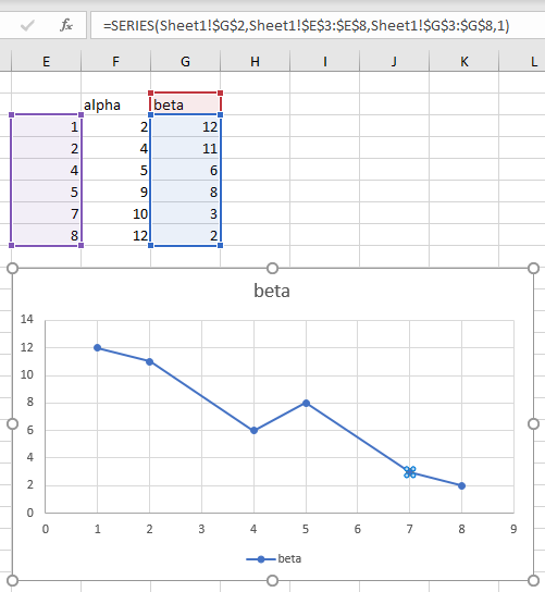
And both of these techniques are easier than going through the whole Select Data > Edit Series routine.

You can modify any of the arguments. You can change the series name, the X and Y values, and even the series number (plot order). You can type right in the formula, and you can use the mouse to select ranges. Just be careful not to break syntax.

You can also add a new series to a chart by entering a new SERIES formula. Select the chart area of a chart, click in the Formula Bar (or not, Excel will assume you’re typing a SERIES formula), and start typing. It’s even quicker if you copy another series formula, select the chart area, click in the formula bar, paste, and edit.

Cell References and Arrays in the SERIES Formula

Normal Cell References

If you are referencing a cell address, you need to qualify the address with the worksheet name, Sheet1!$F$2. If you try to enter an unqualified reference, $F$2, Excel will give you a warning:

The SERIES formula always uses absolute references, Sheet1!$F$2 as opposed to Sheet1!F2. If you enter a relative reference, Sheet1!F2, Excel will automatically convert it to an absolute reference without any hassle.

Fragmented Ranges

The ranges used for X or Y Values do not need to be contiguous. The following formula is perfectly valid. Both the X Values and Y Values consist of ranges with two areas, with the two areas enclosed in parentheses.

=SERIES(Sheet1!$F$2,(Sheet1!$E$3:$E$5,Sheet1!$E$7:$E$9),(Sheet1!$F$3:$F$5,Sheet1!$F$7:$F$9),1)

I made use of this trick in Add One Trendline for Multiple Series, where I build an uber-formula containing data from all series in a chart (such as the formula below, for three series), and add a trendline that fits all of this data.

=SERIES("Combined",(Sheet1!$B$3:$B$11,Sheet1!$D$3:$D$11,Sheet1!$F$3:$F$11),
(Sheet1!$C$3:$C$11,Sheet1!$E$3:$E$11,Sheet1!$G$3:$G$11),4)

Ranges in Other Workbooks

A chart can reference ranges in external workbooks, as long as the ranges are properly references by workbook and worksheet.

=SERIES([SERIESFormula.xlsm]Sheet1!$F$2,[SERIESFormula.xlsm]Sheet1!$E$3:$E$8,[SERIESFormula.xlsm]Sheet1!$F$3:$F$8,1)

Names (Named Ranges)

If your references are Names (Named Ranges), you need to qualify the Name with the scope of the Name, that is, either its parent worksheet or the parent workbook.

=SERIES(Sheet1!TheSeriesName,Sheet1!TheXValues,Sheet1!TheYValues,1)

You can enter the Name qualified by the worksheet, and if the Name is scoped to the workbook, Excel will fix it for you.

=SERIES(SERIESFormula.xlsm!TheSeriesName,SERIESFormula.xlsm!TheXValues,SERIESFormula.xlsm!TheYValues,1)

Note that the Names you use in a SERIES formula cannot begin with the letters C or R (upper or lower case). You can still use these Names, but you need to use the Select Data Source/Edit Series dialogs to add them.

Arrays

When you use a hard-coded array in a SERIES formula, text values must each be surrounded by double quotes, {“D”,”E”,”F”}, while numerical values should not, {4,5,6}. If numbers are surrounded with quotes, {“4″,”5″,”6”}, they will be treated as text labels in the X Values. In an XY scatter chart, they won’t even appear in the chart, but Excel will use counting numbers {1,2,3} for X Values and zero for Y Values.

Using VBA with the SERIES Formula

Knowing how the SERIES formula works, and having a small bit of knowledge VBA, there is no shortage of charting features you can build with VBA.

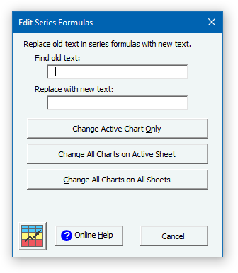
Edit SERIES Formulas (Find-Replace)

There is no built-in Find-and-Replace feature that works with SERIES formulas, but I’ve built my own. It’s based loosely on the following with a lot of error checking that I’ve had to add.

But it’s handy for changing a sheet name (e.g., Sheet1 to Sheet2) or column or row (column $A$ to B or row $5 to 10). Note that I use absolute partial references for columns and rows. Otherwise, I might want to change column S to column Q, and I’d change SERIES to QERIEQ, which would just break.

The following simple macro asks the user for two strings, one to find, and one to change to, and it changes all series in the active chart.

Sub ChangeSeriesFormula_ActiveChart()
  ''' Just do active chart
  If ActiveChart Is Nothing Then
    '' There is no active chart
    MsgBox "Please select a chart and try again.", vbExclamation, _
      "No Chart Selected"
    Exit Sub
  End If

  Dim OldString As String
  OldString = InputBox("Enter the string to be replaced:", "Enter old string")

  If Len(OldString) > 1 Then
    Dim NewString As String
    NewString = InputBox("Enter the string to replace " & """" _
      & OldString & """:", "Enter new string")
    '' Loop through all series
    Dim srs As Series
    For Each srs In ActiveChart.SeriesCollection
      Dim NewFormula As String
      NewFormula = WorksheetFunction.Substitute(mySrs.Formula, _
        OldString, NewString)
      srs.Formula = strTemp
    Next
  Else
    MsgBox "Nothing to be replaced.", vbInformation, "Nothing Entered"
  End If
End Sub

See How To: Use Someone Else’s Macro if you’re not sure how to implement this, or leave a comment below (I check frequently), or shoot me an email. You can modify it to work on all charts on the active sheet, or whatever you like.

This simple code, with about ten times as many lines devoted to checking for user errors and the many eccentricities of Excel, forms the basis of a popular feature in Peltier Tech Charts for Excel.

More VBA & SERIES Formula Examples

I have many more examples of VBA that uses SERIES formulas to get a certain result.

Add Names to Chart Series

Sometimes you are in a hurry to make a chart, and you don’t include the range with the series names. In Simple VBA Code to Manipulate the SERIES Formula and Add Names to Excel Chart Series I have code that determines how the data is plotted, and picks the cell above a column of Y values or to the left of a row of Y values for the name of each series in a chart.

Add Series to Existing Chart

In Add Series to Existing Chart I use VBA to find the last series in a chart, and add another series using the next row or column of data.

Multiple Trendline Calculator

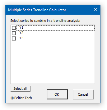
Trendline Calculator for Multiple Series shows code that combines data from multiple series into one big series, and generates a single trendline from this larger series.

Switch X and Y Values (or Axes)

In Switch X and Y Values in a Scatter Chart, I show how to switch the X and Y components of the SERIES formula to switch the X and Y axes of a scatter chart. This is the basis of another feature in Peltier Tech Charts for Excel.

Peltier Tech Consulting Services

I enjoy doing this kind of project. Even with the ribbon components and the dialog, it only takes a few hours. And a few hours of my work will save you time every time you use the result. If you need something like this, send me your requirements and I’ll generate a quote.

Coming to You From…

Sometimes it’s easier to get into blogging from someplace that’s not my office. I used to go to a coffee shop, but that’s so cliché, and it actually doesn’t even work anymore. So today I’m writing from the newest craft brewery in Worcester, Redemption Rock. Maybe I can write it off as a business lunch!

I sampled two very nice IPAs, one very hazy, and two fine stouts, one a nitro stout that was very nice. And they have a nice concoction that combines cold-brewed coffee with the nitro stout, mmmmm.