A reader named Julie has a regular chart that is linked to a pivot table. When the pivot table is pivoted or updated, it may have different numbers of rows and columns, and the chart must be updated manually. Julie asked whether a procedure could be developed to update the chart automatically.
I’ve done this in a number of projects, so I thought I’d illustrate it with a simple example. Let’s start with this dummy data in a list (I’m using Excel 2003).

Insert a pivot table using this data. Drag the Item field to the Rows area, the Category field to the Columns area, and the Value field to the Data area. Simple enough.

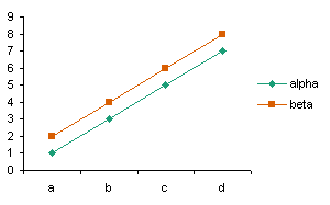
Now create a regular chart from this pivot table, using series in columns, one series per item in the Category field, Category entries (alpha and beta) as series names, and the item names as category (X) axis labels.
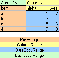
In order to determine which ranges to use for the chart’s source data, it helps to understand what parts of a pivot table are designated as certain ranges. This color coded pivot table illustrates the RowRange, the ColumnRange, the DataBodyRange, and the DataLabelRange. Several of these will be used in the procedure below.
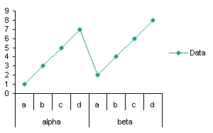
I have set up the macro to put series in columns unless the pivot table DataBodyRange has only one row, in which case there is only one series, and it is plotted by row.
Here is the VBA procedure. Implement it using How To: Use Someone Else’s Macro.
Sub UpdateChartFromPivotTable()
  Dim rValues As Range
  Dim rCats As Range
  Dim rTitles As Range
  Dim cht As Chart
  Dim pt As PivotTable
  Dim chttype As XlChartType
  Dim iSrsIx As Long
  Dim iSrsCt As Long
  Dim iCols As Long
  Dim iRows As Long

  Set cht = ActiveSheet.ChartObjects(1).Chart
  Set pt = ActiveSheet.PivotTables(1)

  Set rValues = pt.DataBodyRange
  On Error Resume Next
  iRows = pt.RowRange.Rows.Count
  iCols = pt.ColumnRange.Columns.Count
  On Error GoTo 0

  If iRows > 0 Then
    Set rCats = Intersect(rValues.EntireRow, pt.RowRange.EntireColumn)
    If iCols > 0 Then
      Set rTitles = Intersect(rValues.EntireColumn, pt.ColumnRange.EntireRow)
      Set rTitles = rTitles.Offset(1).Resize(rTitles.Rows.Count - 1)
    End If
    iSrsCt = rValues.Columns.Count
  ElseIf iCols > 0 Then
    Set rCats = Intersect(rValues.EntireColumn, pt.ColumnRange.EntireRow)
    Set rCats = rCats.Offset(1).Resize(rCats.Rows.Count - 1)
    iSrsCt = rValues.Rows.Count
  Else
    MsgBox "Pivot Table has no fields in Rows area or Columns area.  ", _
        vbCritical + vbOKOnly
    GoTo ExitSub
  End If

  If cht.SeriesCollection.Count > iSrsCt Then
    For iSrsIx = cht.SeriesCollection.Count To iSrsCt + 1 Step -1
      With cht.SeriesCollection(iSrsIx)
        chttype = .ChartType
        .ChartType = xlColumnClustered
        .Delete
      End With
    Next
  ElseIf cht.SeriesCollection.Count < iSrsCt Then
    For iSrsIx = cht.SeriesCollection.Count + 1 To iSrsCt
      cht.SeriesCollection.NewSeries
    Next
  End If

  For iSrsIx = 1 To cht.SeriesCollection.Count
    With cht.SeriesCollection(iSrsIx)
      chttype = .ChartType
      .ChartType = xlColumnClustered
      .XValues = rCats
      If iRows > 0 Then
        .Values = rValues.Columns(iSrsIx)
        If iCols > 0 Then
          .Name = rTitles.Columns(iSrsIx)
        Else
          .Name = "Data"
        End If
      Else
        .Values = rValues.Rows(iSrsIx)
        .Name = "Data"
      End If
      .ChartType = chttype
    End With
  Next

ExitSub:

End Sub
Whenever the pivot table changes you can run this procedure to update the chart. To make it run automatically when the pivot table updates, you could put this event procedure into the code module behind the sheet (to open the sheet’s code module, right click the sheet tab, click View Code).
Private Sub Worksheet_Calculate()
  Application.EnableEvents = False

  UpdateChartFromPivotTable

  Application.EnableEvents = True
End Sub
This procedure runs every time the worksheet calculates, whether or not the pivot table is involved. To redraw the chart only when mandated by pivot table updates, in Excel 2003 and later you can use this event procedure instead:
Private Sub Worksheet_PivotTableUpdate(ByVal Target As PivotTable)
  Application.EnableEvents = False

  If Target.Name = Me.PivotTables(1).Name Then
    UpdateChartFromPivotTable
  End If

  Application.EnableEvents = True
End Sub
You could further modify the code to update different charts which are based on different pivot tables. Modify the indexes in these lines, instead of using “1”.
  Set cht = ActiveSheet.ChartObjects(1).Chart
  Set pt = ActiveSheet.PivotTables(1)
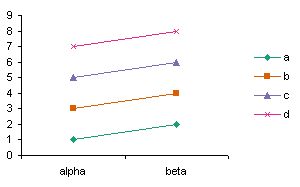
I have run through some permutations of the pivot table and chart:






Bryan Marks says
I have a series of graphs on different worksheets. Each graph is based on a different pivot table. I’m trying to make it so that each graph will automatically be updated if any changes are made to the specific pivot table to which it is tied. For example, the pivot table contains data for all 50 states over ten years. I’d like to see the graph update if someone selects one or multiple states in the pivot table without repeating that exercise by clicking on the graph itself.
I tried using the first macro and then the one below so that only the graph on the same page as the pivot table gets updated, but what is happening is that ALL graphs are getting updated using the same single pivot table data. This is obviously not what I want to happen.
Private Sub Worksheet_PivotTableUpdate(ByVal Target As PivotTable)
Application.EnableEvents = False
If Target.Name = Me.PivotTables(1).Name Then
UpdateChartFromPivotTable
End If
Application.EnableEvents = True
End Sub
Unfortunately, I didn’t understand what you meant with this statement, but this would appear to fix the problem I’m having now: “You could further modify the code to update different charts which are based on different pivot tables. Modify the indexes in these lines, instead of using “1″.” To what do the indexes refer?
Thanks for your help!
Bryan
Jon Peltier says
Bryan –
Right after the sentence you cited, there are two lines of code:
Set cht = ActiveSheet.ChartObjects(1).Chart
Set pt = ActiveSheet.PivotTables(1)
the indexes are the “(1)” in these commands, one for index of the chart object, the other for the index of the pivot table. It might be more robust to name the chart and the pivot table.
Bryan Marks says
Thanks for answering so quickly! Unfortunately, I still have some questions due to my ignorance of macros and VBA:
1. Those two lines of code are already included in the big macro at the top of this post, so does adding them again to the bottom of the macro fix things?
2. I ran a compile on the following code and received an error message saying it was an invalid use of the Me keyword.
3. I’m afraid I still don’t understand what indexes reference. What does “the index of the chart reference” and “the index of the pivot table” mean?
4. Is my problem that the pivot tables are all based on the exact same source data?
5. I hate to ask, but can you put the macro together as it should appear to only update the specific charts associated with a specific pivot table?
Thanks again!
Bryan
Maria says
Hello,
I would like to know how to create multiple different charts from one pivot table.
thanks
Maria
Jon Peltier says
Maria –
See Making Regular Charts from Pivot Tables.
Maria says
Thanks Jon, but my question was about plotting different charts( not including all the data from the pivot table) .what I am thinking is using your script ‘making regular charts from pivot tablse’ but instead of using DataBodyRange, select the rows I want to plot….Do you know how to do it?
Thanks
Cheers,
Maria
Jon Peltier says
Maria –
You asked how to make multiple charts from a pivot table. I assumed you meant multiple charts that did not include the entire pivot table. The article I cited shows a manual procedure (there is no script for this) to make one chart from pivot table without necessarily using all of the pivot table data. You manually select the range for each series in the chart. You would repeat this for each of the multiple charts you wanted.
If you wanted to look at a known subset of the DataBodyRange, you could use
pt.DataBodyRange.Rows(i)
and
pt.DataBodyRange.Columns(j)
for the ith row and jth column.
You may need to build more intelligence into the code, so you select for example the row corresponding to “item c” in case it might not be the 3rd row.
Maria says
Yes you are right but the problem is that I want to select several columns in order to plot them all together in the same graph. I have tried replacing this line:
Set rValues = pt.DataBodyRange
for these ones
Set xValues = pt.PivotFields(“Values”).PivotItems(“Sum of AVG_UL_POWER”).DataRange
Set sValues = pt.PivotFields(“Values”).PivotItems(“Sum of AVG_DL_POWER”).DataRange
Set rValues = Union(xValues, sValues)
but it is not working…
any idea?
thanks,
Maria
Jon Peltier says
Maria –
Oh, I think I get what you want. The problem is that taking the union of some of the Y values may result in a discontiguous range, and you can’t just use row i of a discontiguous set of rows. You need to talk about the range (the union), the areas in the range, the rows in the area. It’s messy, whereas just using the whole DataBodyRange is one area, so it’s neater.
You have to specify data for each series at a time, X values, Y values, and series name. You may as well just do it explicitly instead of in a loop.
Maybe something like this:
Of course, you could always use the filtering in a pivot field to show only the items you want plotted, and it reverts to the example in this article.
Maria says
Thanks Jon,
I have this procedure now… I am trying to plot two charts from the same pivot table.
I am getting an error when trying to populate serie 1 for chart 2,which is in line
.Values = pt.PivotFields(“Values”).PivotItems(“Sum of AVG_MS_DISTANCE”).DataRange
Do you understand why?
Thanks again,
Maria
Sub updatePivotChart()
Dim rCategories As Range
Dim rValues As Range
Dim pt As PivotTable
Dim cht As Chart
Dim pht As Chart
‘ Define the Pivot Table
Set pt = ActiveSheet.PivotTables(“PivotTable1”)
‘ Define the Ranges
With pt.RowRange
Set rCategories = .Offset(1).Resize(.Rows.Count – 1)
End With
‘ Define chart 1 and 2
Set cht = ActiveSheet.ChartObjects(“Chart”).Chart
Set pht = ActiveSheet.ChartObjects(“Chart 1”).Chart
‘ Populate Each Series for chart 1
With cht.SeriesCollection(1)
.Name = “Sum of AVG_DL_POWER”
.Values = pt.PivotFields(“Values”).PivotItems(“Sum of AVG_DL_POWER”).DataRange
.XValues = rCategories
.Border.LineStyle = xlNone
chttype = .ChartType
.ChartType = xlColumnClustered
End With
With cht.SeriesCollection(2)
.Name = “Sum of AVG_UL_POWER”
.Values = pt.PivotFields(“Values”).PivotItems(“Sum of AVG_UL_POWER”).DataRange
.XValues = rCategories
.Border.LineStyle = xlNone
chttype = .ChartType
.ChartType = xlColumnClustered
End With
‘ Populate Each Series for chart 2
With pht.SeriesCollection(1)
.Name = “Sum of AVG_MS_DISTANCE”
.Values = pt.PivotFields(“Values”).PivotItems(“Sum of AVG_MS_DISTANCE”).DataRange
.XValues = rCategories
.Border.LineStyle = xlNone
chttype = .ChartType
.ChartType = xlColumnClustered
End With
With pht.SeriesCollection(2)
.Name = “Sum of INTER_IN_HO_FL”
.Values = pt.PivotFields(“Values”).PivotItems(“Sum of INTER_IN_HO_FL”).DataRange
.XValues = rCategories
.Border.LineStyle = xlNone
chttype = .ChartType
.ChartType = xline
End With
End Sub
Jon Peltier says
It worked for the first chart?
What’s the error (not error number but error description)?
What’s the chart type?
Did the series have any data points before running the code?
Is “Sum of AVG_MS_DISTANCE” spelled correctly?
Is “Sum of AVG_MS_DISTANCE” a visible pivot item?
Maria says
Thanks Jon. The error was because I had not added the series in the chart so now it is working!
The problem with this procedure is that you need to define the chart manually instead of creating it directly with the procedure so now I am trying to do this:
‘ Populate Each Series for chart 1
With ActiveSheet.ChartObjects.Add _
(Left:=100, Width:=375, Top:=75, Height:=225)
.Chart.SetSourceData Source:=Sheets(“Sheet2”).Range(“22B:26B”)
.Chart.ChartType = xlLine
End With
The issue now is if I can choose the data dor the chart as I did in the previous procedure( with pt.PivotFields(“Values”).PivotItems(“Sum of AVG_DL_POWER”).DataRange ).
My try is..
‘ Populate Each Series for chart 1
With ActiveSheet.ChartObjects.Add _
(Left:=100, Width:=375, Top:=75, Height:=225)
.Chart.SetSourceData Source:=pt.PivotFields(“Values”).PivotItems(“Sum of AVG_DL_POWER”).DataRange
.Chart.ChartType = xlLine
End With
But It is not working…
thanks!
Maria
Jon Peltier says
Maria –
If SetSourceData includes any pivot table data, the chart will automatically convert into a pivot chart based on that pivot table.
You have to make sure a blank cell surrounded by blank cells is selected before you use ChartObjects.Add, which will produce a blank chart with no data series. Then you have to add each series:
Also, Range(“22B:26B”) is incorrect. If you want that particular range it is referenced as Range(“B22:B26”). But again, you probably do not want to use SetSourceData.
Maria says
Thanks again!
Maria says
It is me again! Is is posible to create pointers in VBA?
I have a config table with all the parameters in sheet2 of the xlms.
Series Graph Title Legend GRAPH_LOCATION X-Axis
TCH_ASS_FR TCH_Assignment xlLegendPositionBottom DATETIME
TCH_ASS_SUC TCH_Assignment xlLegendPositionBottom DATETIME
TCH_ASS_ATT TCH_Assignment xlLegendPositionBottom DATETIME
And in the previous macro , I would like to automatically create charts when inserting data in the config table. For that, I am trying to get the name from the column ‘Series’ and what is more difficult, get the data from the column of the pivot table which belongs to that name ( In this case ” $Sheet2!A2″= TCH_ASS_FR )
.Name = ” $Sheet2!A2″
.Values = pt.PivotFields(“Values”).PivotItems(” $Sheet2!A2″).DataRange
Any idea?
Thanks again!
Maria
Jon Peltier says
Maria –
Like this?
Dim sName As String
sName = ThisWorkbook.Worksheets(“Sheet2”).Range(“A2”).Value
.Name = sName
.Values = pt.PivotFields(“Values”).PivotItems(sName).DataRange
Maria says
Yes, exactly! THank you!
Maria
Maria says
Hi again, Good morning!
Let’s see if I can get some help this time…I have a pivot table with a filter field called CELL_NAME ..I am doing several charts of each CELL_NAME.
I have the charts appearing in a different sheet(sheet 3) but I want them in a diferent sheet.The problem is that I need the filter field to be in the same sheet as the charts, as it is more user friendly.. so I would need to ‘duplicate’ the filter for CELL_NAME to appear also in the same sheet as the charts.
I have tried with getpivotdata() but no luck and also I am not sure what is that function for..Also, I have thought that maybe it is posible to create a new pivot table and link both somehow…Although I would prefer not having two pivot tables….
any idea?
thanks in advance!!
Maria
Doug Rubin says
First thanks for the intelligent and helpful advice. I was actually able to create a new VBAProject Module, paste in a Macro and then get it to work, when a PivotChart updates. I have never used Excel Macros before so this was a big step.
But (of course), my challenge is a bit different . . . I have a PivotTable . . that then populates another Worksheet of my Workbook . .. and on the same Worksheet as the PivotTable, I have a customized (non-Pivot) Line Graph that is based on a fixed series of cells from the other Worksheet.
The code as described certainly updates the Line Graph, but it updates it using data from the PivotTable directly . . . I want it to use the enhanced values (w. additional data) from the non-Pivot Worksheet. And it does not . . .
So I want the LineGraph to update from the non-Pivot Worksheet whenever the PivotTable is updated. Does that make sense?
Thanks for your suggestions.
Doug
Jon Peltier says
Doug –
You can use the same event that launches the current macro, but link to the other chart and the other data set.
Alberto Basantes says
hi. I have a question.
I have an slicer linked to two pivot tables that generate two regular graphs. I want this code to work everytime I move the slicer and both pivot tables are refreshed, so that both graphs can be updated at the same time.
Meanwhile what I managed to do is instead of using –UpdateChartFromPivotTable– i “Call” the Macro that wrote following this tutorial.
But i dont know if this is the best way to do this.