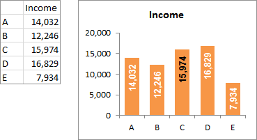
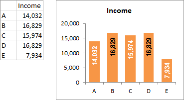
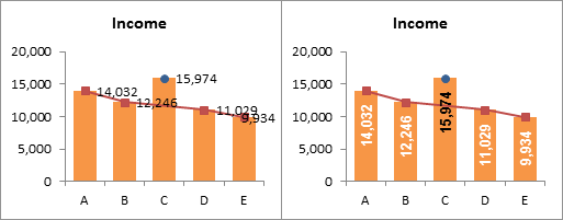
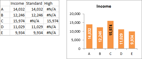
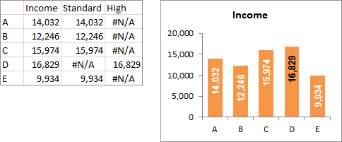
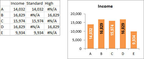
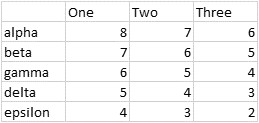
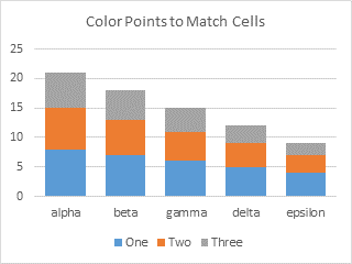
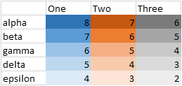
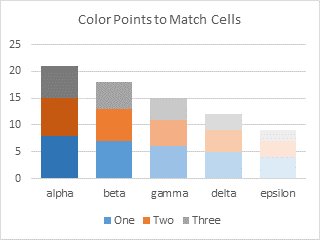
Often you want to add custom data labels to your chart. The chart below uses labels from a column of data next to the plotted values.

When you first add data labels to a chart, Excel decides what to use for labels—usually the Y values for the plotted points, and in what position to place the points—above or right of markers, centered in bars or columns. Of course you can change these settings, but it isn’t obvious how to use custom text for your labels.
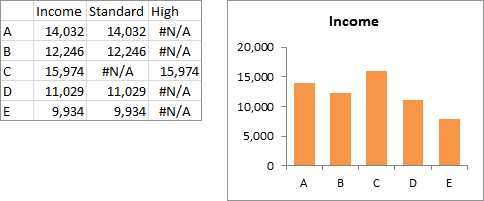
This chart is the starting point for our exercise. It plots simple data from columns B and C, and it displays only the default data labels, showing the Y values of each point.

There are a number of ways to apply custom data labels to your chart:
- Manually Type Desired Text for Each Label
- Manually Link Each Label to Cell with Desired Text
- Use the Chart Labeler Program
- Use Values from Cells (Excel 2013 and later)
- Write Your Own VBA Routines
Manually Type Desired Text for Each Label
The least sophisticated way to get your desired text into each label is to manually type it in.
Click once on a label to select the series of labels.
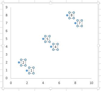
Click again on a label to select just that specific label.

Double click on the label to highlight the text of the label, or just click once to insert the cursor into the existing text.

Type the text you want to display in the label, and press the Enter key.
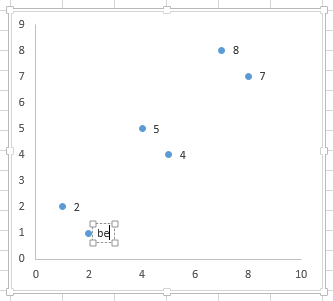
Repeat for all of your custom data labels. This could get tedious, and you run the risk of typing the wrong text for the wrong label (I initially typed “alpha” for the label above, and had to redo my screenshot).
One thing that makes this approach unsophisticated is that the typed labels are not dynamic. If th text in one of the cells changes, the corresponding label will not update.
Manually Link Each Label to Cell with Desired Text
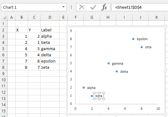
Select an individual label (two single clicks as shown above, so the label is selected but the cursor is not in the label text), type an equals sign in the formula bar, click on the cell containing the label you want, and press Enter. The formula bar shows the link (=Sheet1!$D$3).
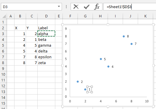
Repeat for each of the labels. This could get tedious, but at least the labels are dynamic. If the text in one of the cells changes, the corresponding label updates to show the new text.
Use the Chart Labeler Program
Brilliant Excel jockey and former MVP Rob Bovey has written a Chart Labeler add-in, which allows you to assign labels from a worksheet range to the points in a chart. It is free for anyone to use and can be downloaded from http://appspro.com. Rob colls it the XY Chart Labeler, but it actually works with any chart type that supports data labels.
When installed, the add-in adds a custom ribbon tab with a handful of useful commands. The tab is added at the end of the ribbon, but being pressed for space I moved it digitally to the beginning.
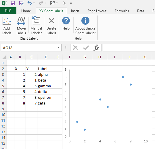
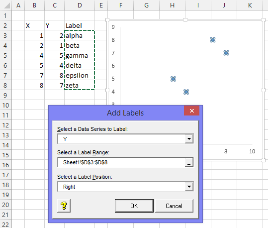
With a chart selected, click the Add Labels ribbon button (if a chart is not selected, a dialog pops up with a list of charts on the active worksheet). A dialog pops up so you can choose which series to label, select a worksheet range with the custom data labels, and pick a position for the labels.
If you select a single label, you can see that the label contains a link to the corresponding worksheet cell. This is like the previous method, but less tedious and much faster.
Use Values from Cells (Excel 2013 and later)
After years and years of listening to its users begging, Microsoft finally added an improved labeling option to Excel 2013.
First, add labels to your series, then press Ctrl+1 (numeral one) to open the Format Data Labels task pane. I’ve shown the task pane below floating next to the chart, but it’s usually docked off to the right edge of the Excel window.

Click on the new checkbox for Values From Cells, and a small dialog pops up that allows you to select a range containing your custom data labels.

Select your data label range.

Then uncheck the Y Value option. I also uncheck the Show Leader Lines option, which is another enhancement added in Excel 2013. Leader lines are hardly ever useful for the charts I make, but many users are happy with them.
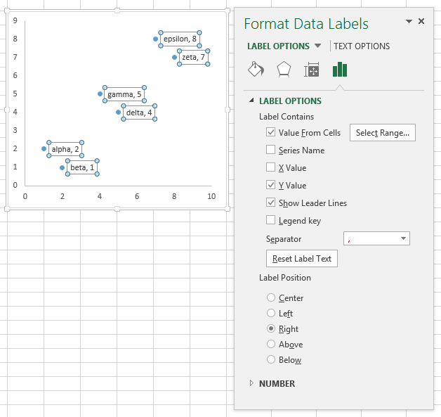
While these data labels are not explicitly linked to worksheet cells as in the previous approaches, they still reflect any changes to the cells that contain the labels.
Write Your Own VBA Routines
I’ve put together a couple little routines that help with data point labeling. These are quick and dirty, because sometimes that’s all that you need. Also, writing your own code allows you to streamline your workflow according to your specific requirements.
Add Data Labels from Range Selected by User
This routine first makes sure a chart is selected, then it determines which series is to be labeled. It asks the user to select a range using an InputBox, and if the user doesn’t cancel it adds a label to the series point by point, linking the label to the appropriate cell.
Sub AddLabelsFromUserSelectedRange()
  Dim srs As Series, rng As Range, lbl As DataLabel
  Dim iLbl As Long, nLbls As Long

  If Not ActiveChart Is Nothing Then
    If ActiveChart.SeriesCollection.Count = 1 Then
      ' use only series in chart
      Set srs = ActiveChart.SeriesCollection(1)
    Else
      ' use series associated with selected object
      Select Case TypeName(Selection)
        Case "Series"
          Set srs = Selection
        Case "Point"
          Set srs = Selection.Parent
        Case "DataLabels"
          Set srs = Selection.Parent
        Case "DataLabel"
          Set srs = Selection.Parent.Parent
      End Select
    End If

    If Not srs Is Nothing Then
      ' ask user for range, avoid error if canceled
      On Error Resume Next
      Set rng = Application.InputBox( _
          "Select range containing data labels", _
          "Select Range with Labels", , , , , , 8)
      On Error GoTo 0

      If Not rng Is Nothing Then
        ' point by point, assign cell's address to label
        nLbls = srs.Points.Count
        If rng.Cells.Count < nLbls Then nLbls = rng.Cells.Count
        For iLbl = 1 To nLbls
          srs.Points(iLbl).HasDataLabel = True
          Set lbl = srs.Points(iLbl).DataLabel
          With lbl
            .Text = "=" & rng.Cells(iLbl).Address(External:=True)
            .Position = xlLabelPositionRight
          End With
        Next
      End If
    End If
  End If
End Sub
Add Data Labels from Row or Column Next to Y Values
This routine first makes sure a chart is selected, then it determines which series is to be labeled. It doesn’t bother the user, instead the routine parses the series formula to find the range containing the Y values, and if this is a valid range, it finds the next column or row, depending on the orientation of the Y values range. The code then adds a label to the series point by point, linking the label to the appropriate cell.
Sub AddLabelsFromRangeNextToYValues()
  Dim srs As Series, rng As Range, lbl As DataLabel
  Dim iLbl As Long, nLbls As Long
  Dim sFmla As String, sTemp As String, vFmla As Variant

  If Not ActiveChart Is Nothing Then
    If ActiveChart.SeriesCollection.Count = 1 Then
      ' use only series in chart
      Set srs = ActiveChart.SeriesCollection(1)
    Else
      ' use series associated with selected object
      Select Case TypeName(Selection)
        Case "Series"
          Set srs = Selection
        Case "Point"
          Set srs = Selection.Parent
        Case "DataLabels"
          Set srs = Selection.Parent
        Case "DataLabel"
          Set srs = Selection.Parent.Parent
      End Select
    End If

    If Not srs Is Nothing Then
      ' parse series formula to get range containing Y values
      sFmla = srs.Formula
      sTemp = Mid$(Left$(sFmla, Len(sFmla) - 1), InStr(sFmla, "(") + 1)
      vFmla = Split(sTemp, ",")
      sTemp = vFmla(LBound(vFmla) + 2)
      On Error Resume Next
      Set rng = Range(sTemp)

      If Not rng Is Nothing Then
        ' use next column or row as appropriate
        If rng.Columns.Count = 1 Then
          Set rng = rng.Offset(, 1)
        Else
          Set rng = rng.Offset(1)
        End If

        ' point by point, assign cell's address to label
        nLbls = srs.Points.Count
        If rng.Cells.Count < nLbls Then nLbls = rng.Cells.Count
        For iLbl = 1 To nLbls
          srs.Points(iLbl).HasDataLabel = True
          Set lbl = srs.Points(iLbl).DataLabel
          With lbl
            .Text = "=" & rng.Cells(iLbl).Address(External:=True)
            .Position = xlLabelPositionRight
          End With
        Next
      End If
    End If
  End If
End Sub








 Jon Acampora writes the blog at

