The xkcd Velociraptor Problem #1
In Substitute, we learn of a substitute teacher’s “real-life” math problems, which include the following:

Ha, ha, funny commentary on a frustrated old substitute math teacher. (Disclosure: my wife is an 8th grade math teacher, and frustrated is often descriptive of her job.)
So how far could you get before you become Velociraptor Chow? Rhett Allain, a science writer at Wired Magazine, shows us how to figure this out in Here’s How to Solve the xkcd Velociraptor Problem With Code. Prof. Allain describes a numerical approach to the problem using some physics and a bit of python code. Essentially you have some initial conditions, such as speed and position of predator and prey, and some boundary conditions, such as acceleration and maximum speed of each. You select a suitably short time increment, compute the speed due to acceleration and distance traveled based on speed, and update the conditions. If the dinosaur hasn’t yet caught the primate, you again increment the time, update the conditions, and so on, until the two participants coincide in space and time.
You could use your best 8th grade algebra (or my wife’s) and compute the solution analytically, but that’s more suited to paper and pencil, not to a computer. And the numerical approach can be applied to many phenomena, physical and other (including financial).
An algebraic solution?
We’ll use Excel to carry out these same calculations, both as a set of worksheet formulas and as a VBA routine.
In his Calvin and Hobbes comic strip, Bill Watterson has touched on velociraptor-human conflict, not as a physics problem but as a solution to an ecological problem (human overpopulation).
Approach 1. Using Excel Table with Simple Formulas
Using an Excel table allows you to make iterative calculations easily. Once you get the formulas right, you can then extend the calculations by adding rows to the table.
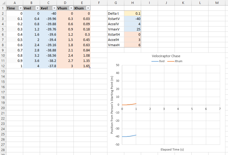
Below is the initial setup of the velociraptor problem. Calculations are compiled in a table in the top left of the worksheet. Parameters for the problem are listed in a range nearby and are used in definitions for Names that make setting up the problem easier (see definitions below). The chart plots positions of the velociraptor and of the human on the Y axis vs. time on the X axis.
This screen shot of Excel’s Name Manager dialog shows the Names which were defined to facilitate calculations. Delta_t is the time increment between calculated time points in the table. XstartV and XstartH are the initial positions of the velociraptor and of the human. AccelV and AccelH are the acceleration for the velociraptor and for the human. VmaxV and VmaxH are the maximum running speeds for the velociraptor and for the human.

The table contains these column formulas:
Time
=IF(ROW()-ROW(Table1[#Headers])=1,
    0,
    OFFSET([@Time],-1,0)+Delta_t)
Vvel (velocity of the velociraptor)
=IF([@Time]=0,
0,
IF(OFFSET([@Vvel],-1,0)>=VmaxV,
VmaxV,
MIN(OFFSET([@Vvel],-1,0)+AccelV*Delta_t,VmaxV)))Xvel (position of the velociraptor)
=IF([@Time]=0,
XstartV,
OFFSET([@Xvel],-1,0)+[@Vvel]*Delta_t)Vhum (velocity of the human)
=IF([@Time]=0,
0,
IF(OFFSET([@Vhum],-1,0)>=VmaxH,
VmaxH,
MIN(OFFSET([@Vhum],-1,0)+AccelH*Delta_t,VmaxH)))Xhum (position of the human)
=IF([@Time]=0,
XstartH,
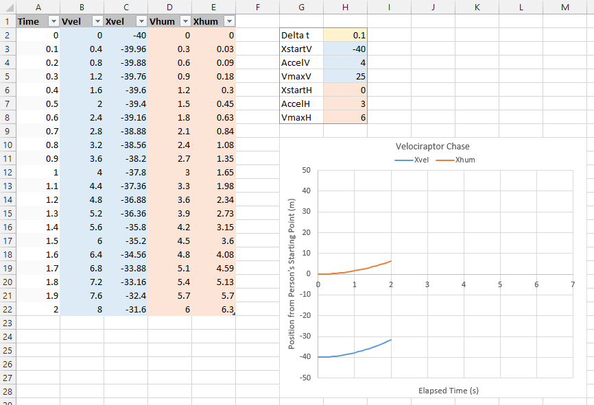
OFFSET([@Xhum],-1,0)+[@Vhum]*Delta_t)This screenshot shows the table populated to an elapsed time of 2 seconds. The human has just reached his maximum velocity, but the velociraptor is still accelerating. The dinosaur has gotten slightly closer to the human.
You can extend the chase by extending the table, simply by clicking on the small angle-iron at the bottom right corner of the tab and dragging it down as far as needed.
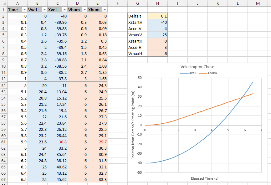
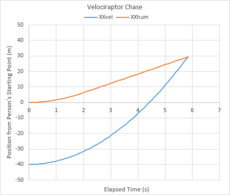
Below, the table has been filled down to 6.5 seconds (the rows between 1 sec and 5 sec have been hidden). We see from the chart that the velociraptor has overtaken the human, and I’ve indicated with red text the row in the table where the position of the velociraptor has first passed the position of the human (row 62, 5.9 sec).
This simplistic model doesn’t stop when the velociraptor reaches his dinner. We need to insert some intelligence into the formulas in our table.
Approach 2. Using Excel Table with More Detailed Formulas
Using a more detailed table allows you to calculate the point of intersection of the paths of the velociraptor and the human, and stop the chase at that time.
Below is the initial setup of the velociraptor problem.
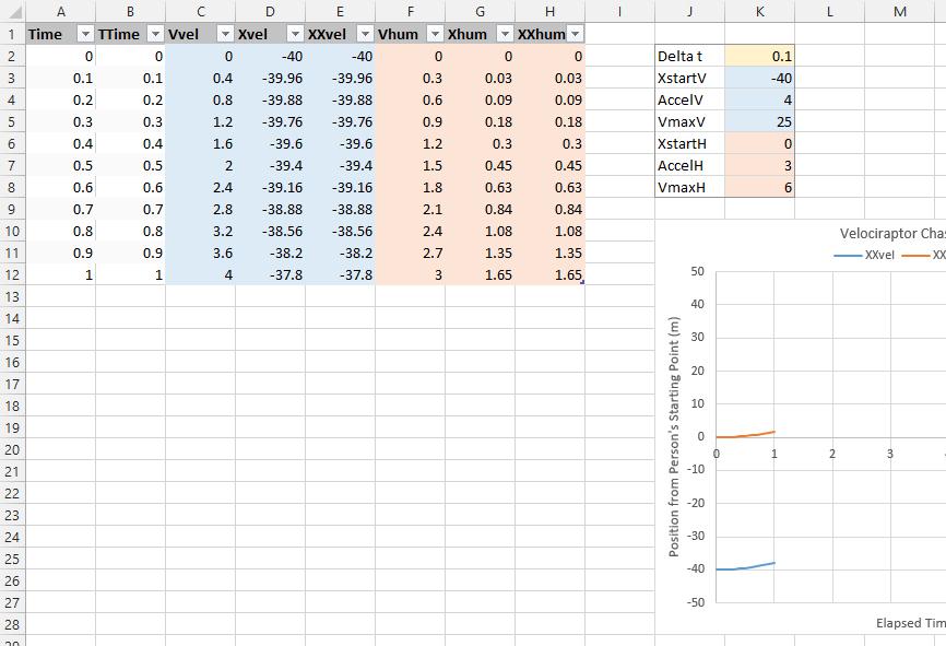
There are a few additional columns:
TTime (adjusted time)
=IF(ROW()-ROW(Table14[#Headers])=1,
    0,
    IF(OFFSET([@TTime],-1,0)<>OFFSET([@Time],-1,0),
       NA(),
       IF([@Xvel]<=[@Xhum],
          [@Time],
          (OFFSET([@Xhum],-1,0)-OFFSET([@Xvel],-1,0))/
            (OFFSET([@Xhum],-1,0)-OFFSET([@Xvel],-1,0)
            -[@Xhum]+[@Xvel])*Delta_t+OFFSET([@Time],-1,0))))
XXvel (adjusted position of the velociraptor)
=IF([@Time]=[@TTime],
[@Xvel],
OFFSET([@Xvel],-1,0)+[@Vvel]*([@TTime]-OFFSET([@TTime],-1,0)))XXhum (adjusted position of the human)
=IF([@Time]=[@TTime],
[@Xhum],
OFFSET([@Xhum],-1,0)+[@Vhum]*([@TTime]-OFFSET([@TTime],-1,0)))The formula for TTime does a lot of work. It’s equal to zero in the first data row, it fills with #N/A after the velociraptor reaches the human, and if the velociraptor catches the human during the current time increment, it interpolates to find the precise time that this happens (see the red entries in row 61).

The chart shows the paths of the predator and prey only up to the point of capture, at 5.8375 sec, or 29.325 m from the human’s initial position.

Approach 3. Using Excel VBA
You can use Excel VBA to solve this velociraptor problem, and animate the chart which illustrates the chase. Initial and boundary conditions are found in the small table in columns G and H.
Columns A through E are the calculations, as in the first approach, except the results are not calculated by worksheet formulas, but instead are calculated by VBA and output to the table as values. These values are plotted in the larger chart.
The small table in columns J through L show the initial and current (i.e., in the most recently calculated iteration) positions of human and velociraptor. These values are plotted in the smaller chart.
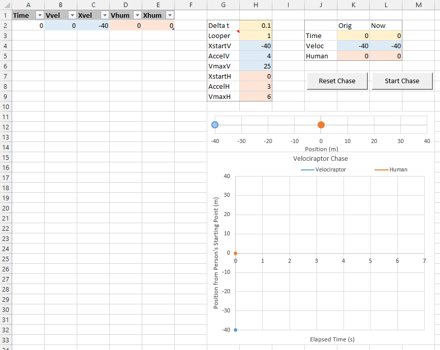
Clicking the Reset Chase button runs the ResetChase procedure (below), which sets conditions back to the start of the chase, by deleting all table rows after the first data row.
Sub ResetChase()
  Application.ScreenUpdating = False
  With ActiveSheet.ListObjects(1)
    Do Until .ListRows.Count = 1
      .ListRows(.ListRows.Count).Delete
    Loop
  End With
  Application.ScreenUpdating = True
End Sub
Clicking the Start Chase button runs the StartChase procedure (below), which starts the chase and runs it until the end.
Sub StartChase()
  Dim tTime0 As Double, tTime1 As Double
  Dim xXhum0 As Double, xXhum1 As Double
  Dim xXvel0 As Double, xXvel1 As Double
  Dim vVhum0 As Double, vVhum1 As Double
  Dim vVvel0 As Double, vVvel1 As Double
  Dim vVmaxH As Double, AccelH As Double
  Dim vVmaxV As Double, AccelV As Double
  Dim DeltaT As Double, DDelTT As Double
  Dim iDelay As Long, iLooper As Long
  Dim ws As Worksheet

  ResetChase

  ' initialize
  Set ws = ActiveSheet
  tTime0 = 0
  iLooper = ws.Range("Looper").Value2
  xXhum0 = ws.Range("XstartH").Value2
  xXvel0 = ws.Range("XstartV").Value2
  vVhum0 = 0
  vVvel0 = 0
  vVmaxH = ws.Range("VmaxH").Value2
  vVmaxV = ws.Range("VmaxV").Value2
  AccelH = ws.Range("AccelH").Value2
  AccelV = ws.Range("AccelV").Value2
  DeltaT = ws.Range("Delta_t").Value2

  ' loop
  Do
    tTime1 = tTime0 + DeltaT

    ' calculate human velocity and position
    If vVhum0 >= vVmaxH Then
      vVhum1 = vVmaxH
    Else
      vVhum1 = vVhum0 + AccelH * DeltaT
      If vVhum1 > vVmaxH Then
        vVhum1 = vVmaxH
      End If
    End If
    xXhum1 = xXhum0 + vVhum1 * DeltaT

    ' calculate velociraptor velocity and position
    If vVvel0 >= vVmaxV Then
      vVvel1 = vVmaxV
    Else
      vVvel1 = vVvel0 + AccelV * DeltaT
      If vVvel1 > vVmaxV Then
        vVvel1 = vVmaxV
      End If
    End If
    xXvel1 = xXvel0 + vVvel1 * DeltaT

    ' has velociraptor caught human?
    If xXvel1 > xXhum1 Then
      DDelTT = DeltaT * (xXhum0 - xXvel0) / _
          ((xXhum0 - xXvel0) + (xXvel1 - xXhum1))
      tTime1 = tTime0 + DDelTT
      xXhum1 = xXhum0 + vVhum1 * DDelTT
      xXvel1 = xXvel0 + vVvel1 * DDelTT
    End If

    ' add new time point data to row below table
    With ws.ListObjects(1)
      .ListRows(.ListRows.Count).Range.Offset(1).Value = _
          Array(tTime1, vVvel1, xXvel1, vVhum1, xXhum1)
    End With

    ' exit if we're done
    If xXvel1 >= xXhum1 Then
      Exit Do
    End If

    ' build in delay if animation runs too quickly on screen
    For iDelay = 1 To iLooper
      DoEvents
    Next
    DoEvents

    ' persist previous loop's data
    tTime0 = tTime1
    vVhum0 = vVhum1
    xXhum0 = xXhum1
    vVvel0 = vVvel1
    xXvel0 = xXvel1
  Loop

End Sub
As the VBA code runs and data is added to the table, you can watch the chase progress in the two charts. Here is the chase after two seconds.

Here is the chase after four seconds.

And here is the chase at its conclusion.

Same result as the table based approaches, except for the added benefit of watching the animation as the VBA calculations proceed.
VBA: Accuracy vs. Calculation Load
Obviously the accuracy of our numerical solution depends on the size of the time increment we use in our calculations. If we take smaller time increments, we can reduce the error resulting from treating nonlinear behavior (acceleration) as linear. On the other hand, taking smaller time increments means our program has to make more calculations, and therefore it will run more slowly.
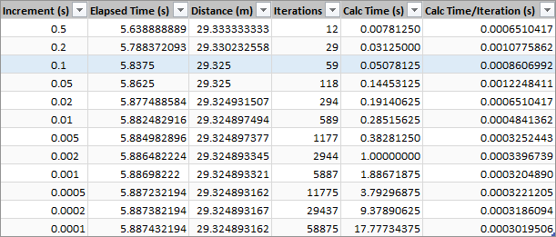
I ran a modified StartChase procedure to determine how time increment size affected elapsed time, distance, number of iteractions, total calculation time, and calculation time per iteration. I turned off screen updating during this procedure and did not output the results of each increment to the worksheet, to ignore the time VBA spends communicating with the Excel worksheet.
Here are the effects of increment time on solution accuracy and calculation time. The blue shaded row shows the solution used in the examples above, an increment of 0.1 sec.
We learn some interesting things if we plot this data.
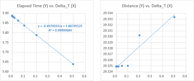
If we plot computed elapsed time to capture of the human vs time increment (Delta_T), we see a straight line with an almost perfect correlation (below left). The computed elapsed time gets closer and closer to the Y intercept as the time increment decreases. We could say that this Y-intercept is the actual time of capture, and our solutions get closer and closer to predicting it as the error in the incremental calculations is minimized. In fact, the difference between the time increment used above (0.1 sec) and the Y-intercept is only 0.05 sec. Maybe we can decide that our analytical solution using an increment of 0.1 sec is “accurate enough”.
If we plot distance to capture vs time increment (below right), we see a trend, but not a nice linear trend as with the elapsed time chart. However, we see that for time increments of 0.1 sec or shorter, there is barely any deviation from the 0.1 sec computation of 29.325 m.
Naturally, a smaller time increment will result in more iterations, in an inverse relationship. The chart below left shows a linear scatter chart, which isn’t very interesting; the data for a large increment (0.5 s) is found out on the X axis. Shortening the increment brings the points back along the X axis until they curve around and head up the Y axis. What is happening is shown better in the log-log plot below right. This is a straight line, and the exponent on X is -0.9995, extremely close to the inverse 1/X relationship we expect.

We would expect a similar inverse relationship between total calculation time and time increment. The linear chart below left shows the same axis-hugging behavior as above, and the log-log chart below right gives us another straight line. This one isn’t as perfectly straight, but a regression on the points for smaller increments (filled points) has a strong correlation and a nearly 1/X relationship.
For the time increment of 0.1 sec from the examples above, we have a total calculation time of 0.05 sec, which is pretty fast for an “accurate enough” solution. If we really want more accuracy, we could even go to a 1 sec solution based on a o.oo2 time increment.
Keep in mind that these calculation times are for a modified procedure, not the procedure that updates the table and chart after each calculation increment. Our 0.1 sec time increment may give the solution in 0.05 sec, but the time we spend watching each increment update the table and chart is more like 4 or 5 seconds.

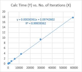
Finally, we see that as the number of iterations increases, the calculation time increases linearly.


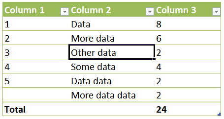
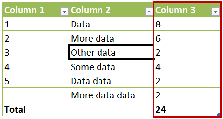
![Table Special Identifier [#All]](https://peltiertech.com/images/2015-06/SI_All.png)
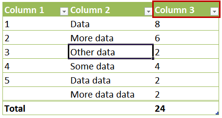
![Table Special Identifier [#Headers]](https://peltiertech.com/images/2015-06/SI_Headers.png)
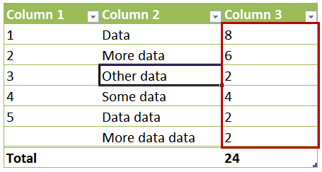
![Table Special Identifier [#Data]](https://peltiertech.com/images/2015-06/SI_Body.png)
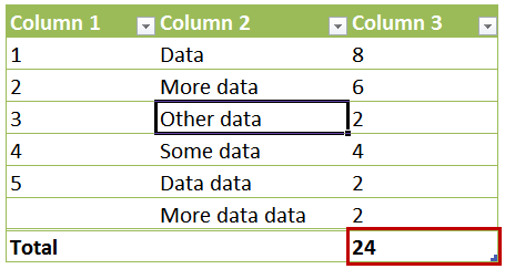
![Table Special Identifier [#Totals]](https://peltiertech.com/images/2015-06/SI_Totals.png)
![Table Special Identifier @ or [#This Row]](https://peltiertech.com/images/2015-06/SI_ThisRow.png)
