A reader encountered problems applying conditional formatting to a pivot table. I tried it myself, using the same kind of formulas I would have applied in a regular worksheet range, and had no problem. The reader responded that he was having problems in Excel 2007, and I was using 2003. Apparently in 2003 the conditional formatting is preserved when the table is refreshed, but in 2007, the CF in the data range is wiped out.
Well, this is just the type of thing Bill gates invented Visual Basic for. I’ll apply an approach related to that in my VBA Conditional Chart Formatting series: VBA Conditional Formatting of Charts by Series Name, VBA Conditional Formatting of Charts by Category Label, and VBA Conditional Formatting of Charts by Value, with a little help from Referencing Pivot Table Ranges in VBA. I’ll use arbitrary data and an arbitrary condition for the example.
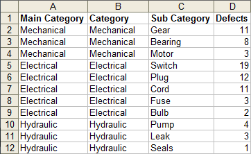
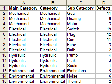
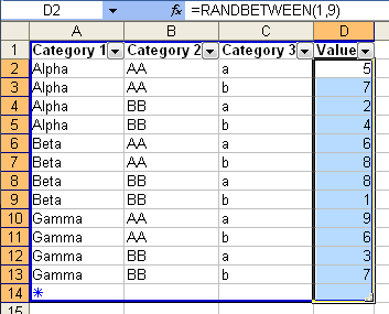
Here is a data source for a simple pivot table. The entire range of values in column D consists of random integers between 1 and 9, and there are three categories by which they can be sorted.
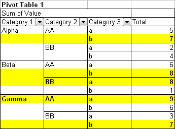
The first pivot table, PivotTable1, has the category fields all placed in the rows area. I manually typed the name “Pivot Table 1” in the cell above the pivot table.

Tip: To name a pivot table, right click on the table, choose Table Options, and edit the name in the first line of the dialog.
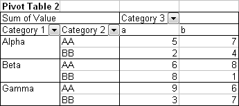
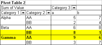
The second pivot table, PivotTable2, has one category in the columns area, so the values are separated into two columns.
I used the following VBA procedure to apply bold text and yellow fill formatting to rows in PivotTable1 if the value in the Total column is 7 or greater. We are testing the entire DataBodyRange, which is one column wide.
Sub FormatPT1()
  Dim c As Range
  With ActiveSheet.PivotTables("PivotTable1")

    ' reset default formatting
    With .TableRange1
      .Font.Bold = False
      .Interior.ColorIndex = 0
    End With

    ' apply formatting to each row if condition is met
    For Each c In .DataBodyRange.Cells
      If c.Value >= 7 Then
        With .TableRange1.Rows(c.Row - .TableRange1.Row + 1)
          .Font.Bold = True
          .Interior.ColorIndex = 6
        End With
      End If
    Next

  End With
End Sub
I used the next procedure to apply the same formatting to PivotTable2 rows if the value in column a under Category 3 is 7 or greater. The DataBodyRange is two columns wide, for pivot items “a” and “b”. To test against pivot item “a”, we test the pivot item’s DataRange.
Sub FormatPT2()
  Dim c As Range
  With ActiveSheet.PivotTables("Pivottable2")

    ' reset default formatting
    With .TableRange1
      .Font.Bold = False
      .Interior.ColorIndex = 0
    End With

    ' apply formatting to each row if condition is met
    For Each c In .PivotFields("Category 3").PivotItems("a").DataRange.Cells
      If c.Value >= 7 Then
        With .TableRange1.Rows(c.Row - .TableRange1.Row + 1)
          .Font.Bold = True
          .Interior.ColorIndex = 6
        End With
      End If
    Next

  End With
End Sub
The two procedures above belong in a regular code module.
Here is PivotTable1 with the conditional formatting applied.
Here is PivotTable2 with the same formatting applied.
Note that refreshing the pivot tables changes values but does not automatically reformat the tables. You have to manually rerun the VBA routines, or capture the PivotTableUpdate event:
Private Sub Worksheet_PivotTableUpdate(ByVal Target As PivotTable)
  Select Case Target.Name
    Case "PivotTable1"
      FormatPT1
    Case "PivotTable2"
      FormatPT2
  End Select
End Sub
This procedure goes in the code module for the worksheet that contains the pivot tables. To access this module easily, right click on the sheet tab, and choose View Code. If you use this approach, you can put the first two procedures into the worksheet’s code module, instead of a regular module.


