Guest Post

If you work with any type of data, then you know that rarely does it come perfectly in the format you need. Power Query (also called Get & Transform in Excel 2016) is the solution to this problem. Power Query is an amazing ETL tool (Extract, Transform, and Load). If you’re not using it then you’re missing out on the best new feature in Excel.

For a more detailed look at what Power Query is and what you can do with it, check out this Introductory Guide to Power Query.

Power Query can connect to many different types of data, but in this post we’ll take a look at importing data from an Excel workbook and doing some basic data cleansing transformations on some messy data.

The Data

For this post, I’ve prepared some fake sales data (download This Week’s Garbage Data File.xlsx to follow along with the example). It’s presented in a typical fashion which is human readable, but not great for any type of further analysis. In this post, we’ll explore how we can use Power Query to get this data into a standard tabular format which will help facilitate any analysis done later on.

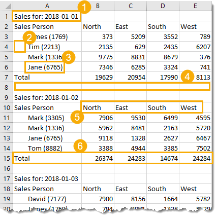
There are a few problems with the data we want to import, and we’ll need to fix them before our data is ready to use.

1. The data has been summarized by date, but the date pertaining to each set of sales only appears once as a heading.
2. There are leading spaces in front of the sales person which will need to be removed.
3. The name of the sales person and their employee ID number have been concatenated together.
4. There are rows of spaces throughout the data that will need to be removed.
5. Sales for the different regions have been pivoted across four different columns. We will want our sales in one column with an extra column defining the region.
6. We have total rows for each of the sections of data that will need to be removed.

Importing Our Data

The first step we need to take is to import our data.

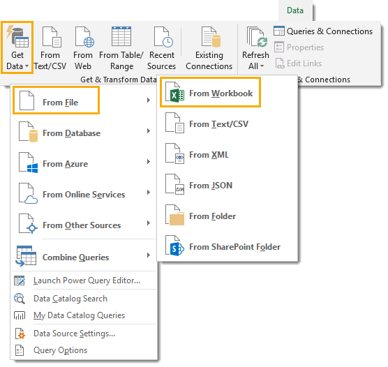
Go to the Data tab and press the Get Data command then choose From File and then From Workbook in the resulting menus.

A file picker menu will appear and we can then navigate to the Excel file we want to import.

Once we’ve picked the file to import, we will be presented with the Navigator window. This will allow us to select the Sales sheet from our workbook which contains the data we want to import. A preview of the data can be seen on the right hand side when selecting sheets.

If our workbook had more than one sheet of data which we wanted to import, we can select multiple sheets using the Select multiple items check box. This would create a separate query for each of the sheets selected and save going through the first couple steps individually.

Now we can either choose to Load the data or Edit it. If we choose to load it, then it will load into an Excel Table with no transformations applied. We want to edit it, this is where we’ll be able to apply our data cleaning transformations. Note: In some builds of Excel, the Edit button is labeled Transform Data.

Press the Edit button and this will open up the Power Query editor.

The Power Query Editor

 

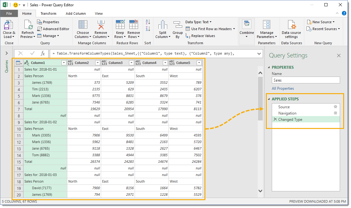
We are now inside the Power Query editor and we can begin building our data transformation to get our data into proper tabular format.

Any transformations you apply to the data will appear as a step in the Applied Steps area. We can step forward and backward through the query by clicking on any of the steps listed in this area.

On the left side of each step is an X that can be used to delete a step and on the right there is a settings icon which can be used to edit the step.

Getting the Date into its Own Column

The first thing we’ll do in our transformation is get the date associated with each section into its own column. Notice that each of these date headings in our data is separated with a colon. Since no other data in this column apart from the dates have a colon, we can use it as a delimiter to split out the data.

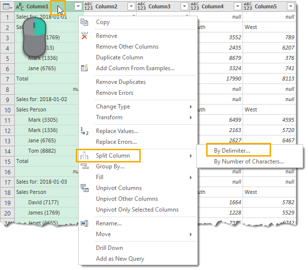
To split this data out, right click on the column heading then select Split Column and then choose By Delimiter.

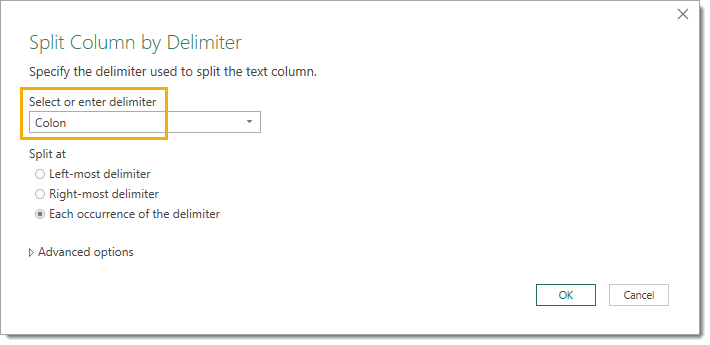
Select Colon from the list of delimiters and press the Ok button.

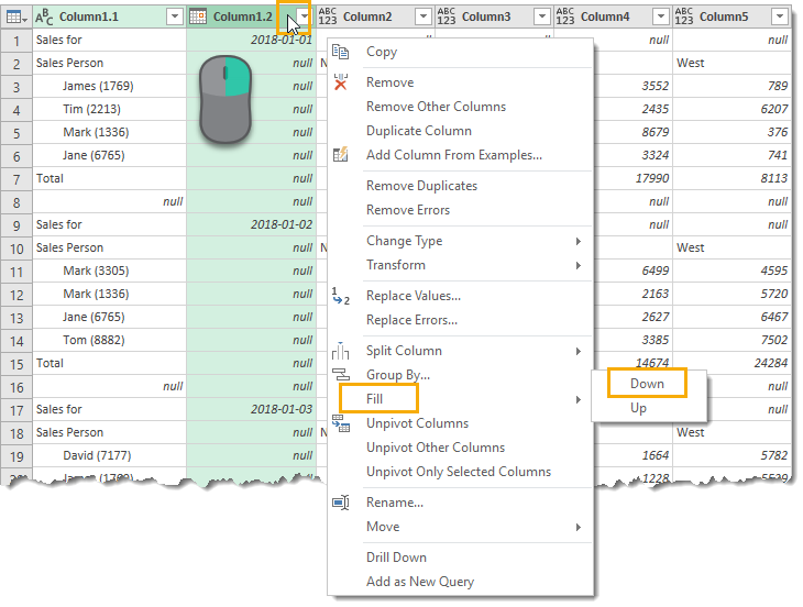
Now we have a new column with dates followed by a series of null values until the next date. Right click on the new column and select Fill then choose Down. This will fill the dates down the column replacing the null values with the date from above.

Split Name and Employee Number

In the next step we’re going to split out the sales persons name and their employee number. The name and employee number are always separated by an opening parenthesis so we’ll use that as the delimiter to split the column.

This assumes that an opening parenthesis will only ever appear in our first column when it is separating the employee number.

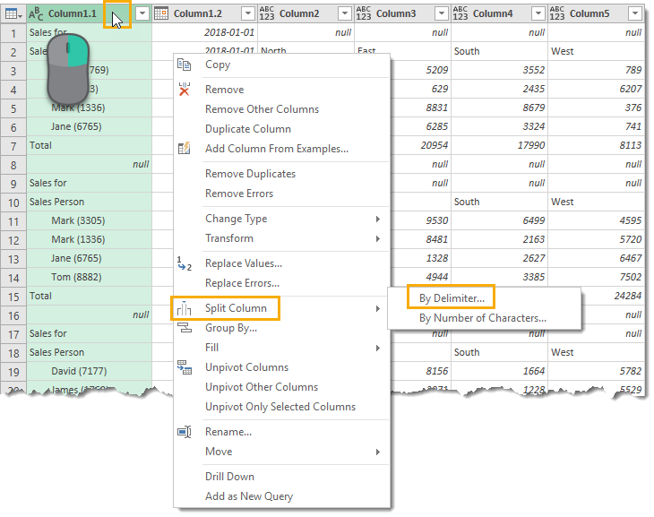
Now we right click on the first column and select Split Column then choose By Delimiter.

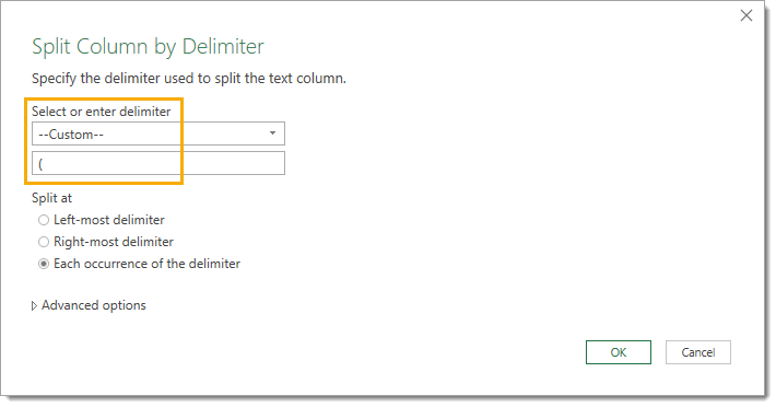
This time we need to use a Custom delimiter since the opening parenthesis is not a standard option. Add in the “(” and press the OK button.

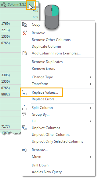
Notice that our new column with the employee number still has the closing parenthesis. We’ll need to clean this up. We can right click on the column and select Replace Values from the menu. Then we can replace the “)” character with nothing. This will remove it from our data.

Remove the Leading Spaces for the Name

Now we can remove the useless leading spaces that were used for indentation in the presentation of the data.

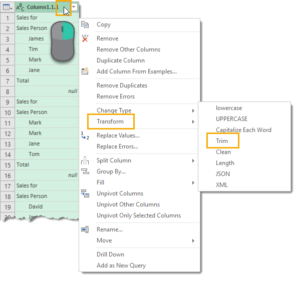
We just need to right click on the column and select Transform and then Trim. This will remove any leading or trailing space characters from our data.

Remove Unnecessary Rows

We’re now ready to remove the unnecessary rows in our data including the total rows and blank rows from our original data file. We also have some rows that are now useless as we’ve already extracted the useful data from them. We can remove all of these rows in the one step.

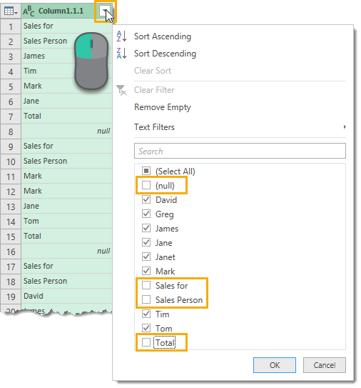
In fact, we’ll be able to do this by filtering on the first column. Click on the filter icon on the right side of the column heading and then deselect the useless rows (null, Sales for, Sales Person, and Total).

You might be asking why we filtered out the row containing Sales Person. Doesn’t that row contain useful column heading information? Couldn’t we use that and promote it to the column headings?

Yes it does, but we can’t use it to promote to column headers because one of the values in that row is the date from the first step in our transformation. That value will likely change if we’re importing a different set of data with this query.

If we were to promote it to a column heading then we’d have a column heading with the label “2018-01-01”. Any further step that references this column, would be referencing this value which won’t exist. This is were our query would break.

Instead we’ll remove this row and rename our current generic column headings to avoid this problem.

Rename Column Headings

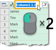
Now we can rename all our columns to their appropriate names. Double click on the current column name to rename a column. We’ll name these Sales Person, Employee ID, Date, North, East, South and West going from left to right.

Unpivot the Region Columns

Now we have an almost tabular set of data. The only thing that remains is to unpivot our four region columns. All the values in these columns represent the same metric of sales and should be in one column with another column that tells us what region the sales amount was from.

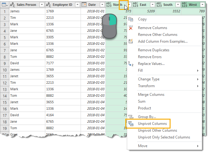
Select the North, East, South and West columns by holding Ctrl and clicking on each heading. You can also select the first (North) column then hold Shift and select the last column (West). Now right click on any of the column headings and select Unpivot Columns.

This will result in two columns called Attribute and Value. We can rename these to Region and Sales respectively.

Change Data Types

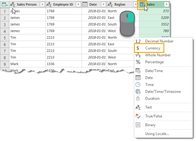
Now our data is just about ready. At the end of any data transformation, it’s good practice to change the data types of columns to the appropriate type.

For the most part our data has the right data types, but our Sales column can be changed to a currency type. Click on the data type icon on the left side of the column heading and select the Currency type from the menu.

Close and Load the Query

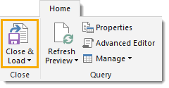
Now that our data transformation is complete, we are going to need to save our query. Go to the Home tab in the query editor and press the Close & Load button. Just remember, you’re still going to need to save the workbook when you’re done in the query editor.

Clicking on the top part of the close and load button will load the data into a new sheet in an Excel table. You can also click on the lower part of the button and select Close & Load To to open the Import Data dialog for more loading options like loading the data directly into a pivot table or into the data model.

For now, we’ll just load the data into a table.

Now we’ve got our data in a ready to use tabular format!

Updating the Query for New Data

Now what happens when we get new data? (Download This Week’s Garbage Data File.xlsx to try this.)

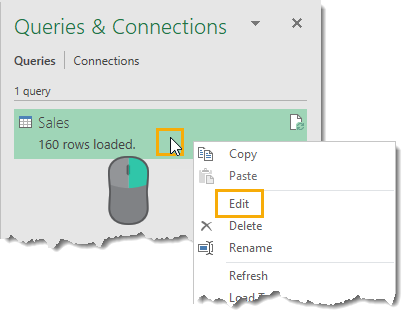
We can use this query again to transform that data. Go to the Data tab and press the Queries & Connections button. Then right click on the query and choose Edit.

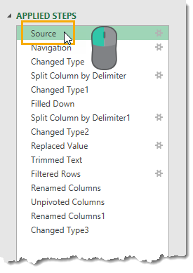
Now we can navigate to the Source step in the Applied Steps area.

Replace the source location in the formula bar with the path and file name of the new data and press the Enter button to confirm the changes. Then we can close and load the query. Our data will update based on the new file!

Note, this will overwrite the previous data, so if we want to retain the old transformed data we’re going to need to create a copy of the workbook before performing these updating steps.

Conclusions

Everything we did in this transformation was using the basic point and click interface in the Power Query editor. Once you get the hang of it, making queries to shape your data into the format you want becomes super easy. No workbook formulas, no difficult VBA and no copying and pasting required.

The best part is, if we need to repeat this transformation with another similar data set, then we can update the file path in the query and press the refresh data button and our new data will be transformed and loaded into Excel. Our messy data problem has become a simple refresh.

This is why Power Query is the best new feature in Excel that you need to start using.

About the Author

John MacDougall is a Microsoft MVP and former actuary who currently works on data analysis and debugging code at an ad tech company. He shares his knowledge and passion for Excel and Power BI through his website How To Excel.