Structured Referencing to Identify Parts of Excel Tables

Guest post by Zack Barresse & Kevin Jones
Data Automation Professionals, LLC

Zack and Kevin are VBA ninjas who have been helping people around the internet for several years. They’ve combined resources and started a company, Data Automation Professionals, which helps Excel users automate simple to complex tasks, consults on projects, and teaches the world VBA. Zack has been hanging around forums like Mr Excel and VBA Express for several years, and maintains the blog at exceltables.com. Kevin is an engineer who has been spotted around the net using the online moniker ‘zorvek’. Together they’ve written a book on Excel Tables: A Complete Guide for Creating, Using and Automating Lists and Tables.

With the introduction of Tables in Excel 2007 (Tables are a re-invention of Lists, introduced in Excel 2003), we were also provided a new syntax for referencing Tables and the parts within those Tables. This new syntax is called structured referencing. The reason a new referencing method is required is because Tables are very dynamic, and the traditional cell referencing syntax would not allow robust referencing without clever use of functions as Tables as data is added and removed. As you will see in this article, structured referencing is a very powerful tool that makes your formulas dynamic while maintaining significant simplicity. If you’re not familiar with Tables, a good starting point is this blog post (with video) by Excel MVP Jon Acampora.

Tables play an integral part of modern Excel. They’re very organized, controlled, and most importantly, they have rules. These allow for a lot of built-in functionality previously unavailable. Functionality such as good data structuring, dynamic chart ranges, dynamic PivotTable sources, etc. Additionally there is some default behavior which can be nice such as banded rows and columns, cell formatting that is added to every new row of a table, and new rows auto-populating with formulas.

All examples in this article are for Excel 2010 and later. There is a slight difference between using structured referencing in Excel 2010 and Excel 2007—Excel 2007 is not covered in this article. For the purposes of discussion, the traditional method of referencing cells (i.e. A1, A2, B1:B100, A2:D100, etc.) is referred to as standard referencing.

Structured Referencing

Before we get too in-depth here, let’s make sure we have a good understanding of what is meant by structured referencing. Structured referencing makes it easier and more intuitive to work with cell references in Tables. It allows you to reference a Table’s parts such as the columns, header rows, and total rows without using standard referencing (R1C1 or A1 syntax) but rather by using the Table’s name and other constants such as column header values which makes references easier to read because recognizable names are used. This eliminates the need to use complex formulas or rewrite formulas when the Table structure is changed or data is added or removed. Formula audits are also made much easier.

Let’s look at a quick example of referencing the hours, let’s say this is stored in column A, and the rate, stored in column B. The standard referencing formula to calculate the total billable amount in row 2 is:

=A2*B2

The structured referencing formula in row 2 (and in all other rows) is:

=[@Hours]*[@Rate]

As you can see, with structured referencing it is much clearer what the formula is doing than with standard referencing. With standard referencing, we have to navigate to the source to determine what, exactly, is in cell A2 and B2. With structured referencing, we have greater transparency with makes development, maintenance, and auditing easier. In today’s world of Excel, with groups like EuSpRIG and heightened auditing and maintenance requirements, transparency in spreadsheets is as important as it’s ever been, and structured referencing goes a long ways to assist.

In the examples below, we will look at a simple Table which has three columns and six rows, with both the header and total rows showing. The image below is used for the next examples.

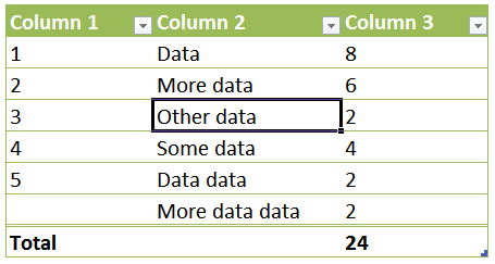
Before we get too in-depth on how the referencing actually takes place, there are a few rules to structured referencing which must be identified. In any single structured reference you may have a

• Table name,
• special identifier, or
• column name.

Generally only the column name is required, but every structured reference will have some combination of these three elements. Below are the basic rules of when to use these elements.

• The Table name used if
  • more than one column of a Table is being referenced, or
  • the column is being referenced from outside of the Table.
• A special identifier is used if a specific part of the Table is being referenced, i.e. the total row.

A key part of structured referencing is the use of square brackets. Square brackets are used to identify a reference as a structured reference versus a standard reference. Every structured reference (except the Table name itself) is enclosed in a set of square brackets. There are two occasions where you will have an additional set of square brackets.

Single-column cell reference

Column name of “Column” (no quotes used as the cell value) has a reference of:

[@Column]

Column name of “A Column” (no quotes used as the cell value—note the space) has a reference of:

[@[A Column]]

Multi-column cell reference

TableName[@[Column1]:[Column2]]

In a multiple column reference, Excel will automatically place a separate set of square brackets around each column name regardless of whether or not there is a space or other special character in the name, as well as append the Table name to the reference. This is to identify it as an individual column within a multiple column reference.

Additionally, below are the characters which Excel identifies and automatically puts an additional set of square brackets around.

• Space ( )
• Line feed
• Carriage return
• Comma ( , )
• Colon ( : )
• Period ( . )
• Left bracket ( [ )
• Right bracket ( ] )
• Pound sign ( # )
• Single quotation mark (apostrophe) ( ‘ )
• Quotation mark (  )
• Left curly bracket (brace) ( { )
• Right curly bracket (brace) ( } )
• Dollar sign ( $ )
• Caret ( ^ )
• Ampersand ( & )
• Asterisk ( * )
• Plus sign ( + )
• Minus sign ( – )
• Equal sign ( = )
• Greater than ( > )
• Less than ( < )
• Division ( / )

This Row

The ampersand character (@) is used to identify “This Row” in a structured reference. This is also known as the implicit intersection of the row in which the reference resides.

Special Characters

Excel uses special characters to qualify structured references (discussed later in more detail) and, when these characters are included as part of a column name, they need to be “escaped” so that Excel does not interpret it as a special reference qualifier. The apostrophe ( ‘ ) is used for this escaping.

Below is a list of all special characters used to qualify structured references and must be preceded by an apostrophe when part of a column header.

• Left bracket ( [ )
• Right bracket ( ] )
• Pound sign ( # )
• Single quotation mark (apostrophe) ( ‘ )
• At sign ( @ )

Special Identifiers

When attempting to reference specific parts of a Table, you will need to use a special identifier. There are only five. Let’s take a look at each of them and a picture for visual reference. In the following examples the referenced area is outlined with a red box.

[#All]

[#Headers]

[#Data]

[#Totals]

@ (or [#This Row] in Excel 2007)

Note that when referencing Table parts which are not visible or enabled such as when a header or total row isn’t showing, the reference will evaluate to a reference error (#REF!). Let’s look at an example formula:

=TableName[[#Headers],[Column 3]]

The above formula references the Table named “TableName”, with the special identifier of the header of “Column 3”. This is a single-cell reference. If the header row is showing the result will be the column name or, in this case, “Column 3”. If the header row is not showing the result will be “#REF!”.

This means we can use formulas to tell if a header or total row is visible or not.

Header row visible formula:

=IF(ISERR(TableName[[#Headers],[Column 3]]),"No","Yes")

Total row visible formula:

=IF(ISERR(TableName[[#Totals],[Column 3]]),"No","Yes")

Another Table part which can possibly not exist is the body. It’s important to note this will not affect formula evaluation, but does have a serious impact in VBA which is covered later in this article.

In Data Validation

Using Tables as a source for an in-cell drop down can simplify your spreadsheets, but Table ranges cannot be referenced directly in the data validation source formula. Instead you must name the range and use that name in the validation formula. To do this, navigate to the FORMULAS tab and click ‘Name Manager’, then click ‘New’.

Since the name of any Table must be unique  for the entire workbook, you cannot name a range the same as a Table name. This is why some people either use Hungarian Notation with naming Tables, or preface all Table names with a “t”. For example, if you have a Table with a list of countries, instead of naming the Table “Countries”, you would name it “tCountries”. This way if you wanted to have those countries as a data validation drop-down list, you could name a range of “Countries” which points to the Table range. Here is an example:

Name: “Countries”

Refers to: “=tCountries[Countries]”

In Charts

Putting your data into Tables and using structured referencing makes it easier to create dynamic charts that change as the data in the Table changes. As to not reinvent the wheel, we’ll refer you to Jon Peltier’ great post about this topic Easy Dynamic Charts Using Lists or Tables. The takeaway from the blog post is Tables make great data sources for charts which grow and shrink as the source data set changes. It’s a nice alternative from having to manually create dynamic named ranges.

In Formulas

Putting all of this information into practice can be confusing. Let’s look at some specific structured referencing syntax examples in formulas. Keep in mind that structured references always evaluate to a range of cells and are treated like any other range reference in Excel, so if you’re referencing more than a single cell it must be used as an aggregate, range array, or lookup array, depending on the formula to which they are being passed.

There are five specific locations we can reference:

• Body column
• Entire column
• Column header
• Column total
• Column cell

The examples below assume the Table’s name is “TableName”, using column “Column Name” where applicable.

Specific Column Body or Data Excluding Header and Total Rows

TableName[Column Name]

Specific Column Including Header and Total Rows

TableName[[#All],[Column Name]]

All Data Excluding Header and Total Rows (Data Body)

TableName

All Data Including Header and Total Rows

TableName[#All]

Row Across All Columns

TableName[@]

Row for One Column (Single Cell)

TableName[@[Column Name]]

Header Row Across All Columns

TableName[#Headers]

Header Row for One Column

TableName[[#Headers],[Column Name]]

Total Row Across All Columns

TableName[#Totals]

Total Row for One Column

TableName[[#Totals],[Column Name]]

Let’s assume we have a column in our Table which is titled “Column 3”. Below are examples of the types of structured references we can use to reference specific parts of that column.

Specific Column Body or Column Data Excluding Header and Total Rows

TableName[Column 3]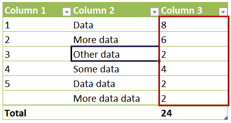

Specific Column Including Header and Total Rows

TableName[[#All],[Column 3]]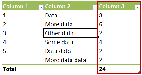

Header Row for One Column

TableName[[#Headers],[Column 3]]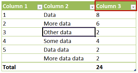

Total Row for One Column

TableName[[#Totals],[Column 3]]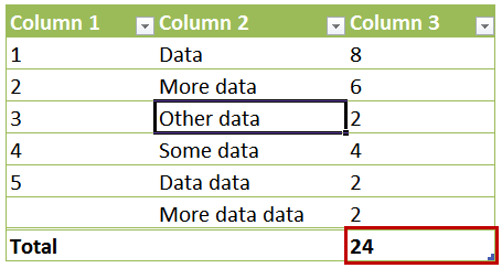

Row for One Column (Single Column Cell)

TableName[@Column 3]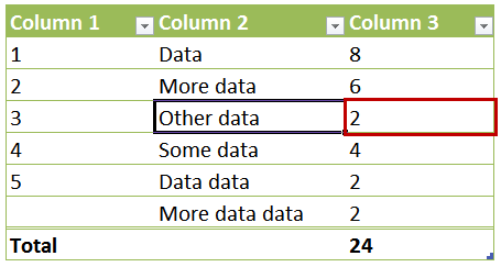

In VBA

There are two basic methods for referencing Tables and parts of Tables from VBA. The easiest is to use the same syntax as described above for formulas where you pass the Table information as a text string to the Range object. The other method is to use the Excel object models ListObject and its child properties and methods. Both are described below.

Using Range and Evaluate

Just as with standard referencing, the Range object evaluates structured references passed as a text string. For example, to reference the body or data portion of “Column 3” in the Table named “TableName” using the Range method:

Range("TableName[Column 3]")

Note that no qualifying worksheet is required because the table name has to be unique across all worksheets. This is the referencing style you will see when using the Macro Recorder.

Using the Object Model’s ListObject

To reference any part of a Table using the Excel object model, we have to first identify the Table object itself. The ListObject object is how Excel exposes a Table in the Excel object model. It is contained in the collection ListObjects which  is a child of the Worksheet object. Use this syntax to reference a specific Table on a worksheet:

ThisWorkbook.Worksheets("Sheet1").ListObjects("Table1")

ListObjects, being a collection of list objects or Tables, can also be accessed with an index number:

ThisWorkbook.Worksheets("Sheet1").ListObjects(1)

The index number of the Table is the order in which it was created on the worksheet and is a read-only property.

Once we have the Table’s ListObject object we can access and manipulate any part of that Table. The more commonly used properties and methods are discussed below. Each example starts with this code:

Dim Table1 As ListObject
Set Table1 = ThisWorkbook.Worksheets("Sheet1").ListObjects("Table1")

Range Property

The Range property returns the entire Table as a range object including the header and total rows.

Dim Table1Range As Range
Set Table1Range = Table1.Range

HeaderRowRange Property

The HeaderRowRange returns the Table’s header row as a Range object. The range is always a single row – the header row – and extends over all Table columns. When the header row is not showing this property returns Nothing.

Dim Table1HeaderRowRange As Range
Set Table1HeaderRowRange = Table1.HeaderRowRange

DataBodyRange Property

The DataBodyRange returns the Table’s body as a Range object. The range is every row between the header and the total row and extends over all Table columns.

Dim Table1DataBodyRange As Range
Set Table1DataBodyRange = Table1.DataBodyRange

When the Table does not contain any rows the DataBodyRange property returns Nothing. This may be confusing when looking at the worksheet as it will appear as if a single row exists. This is the only case when the property InsertRowRange returns a range which can be used to insert a new row. Effectively InsertRowRange and DataBodyRange are equivalent.

TotalRowRange Property

The TotalRowRange returns the Table’s total row as a Range object. The range is always a single row – the total row – and extends over all Table columns. When the total row is disabled this property returns Nothing.

Dim Table1TotalRowRange As Range
Set Table1TotalRowRange = Table1.TotalRowRange

InsertRowRange Property

The InsertRowRange returns the Table’s current insertion row as a Range object only when the Table DataBodyRange object is Nothing (the Table has no data rows); it’s Nothing when the DataBodyRange is a Range (the Table has one or more data rows). While this range was always the last data row in Excel 2003 (the row with the asterisk), it was partially depreciated in Excel 2007 and remains so in 2013. In Excel 2007 and later versions it only returns the first data row and only when the Table does not contain any data. Otherwise it returns Nothing.

Two additional properties or collections provide access to the rows and columns in the Table. Each collection provides access to all of the ListRow and ListColumn objects in the Table. Each ListRow and each ListColumn object has properties and methods.

ListRows Property

The ListRows property returns a collection of the rows in the Table’s DataBodyRange as a ListRows object type. It behaves very much like a Collection object and contains a collection of all the ListRow objects. Rows are referenced only by a one-based index number relative to the first row. An empty Table has no rows. The ListRows.Add method can be used to insert new rows.

Debug.Print "The Table has " & Table1.ListRows.Count & " rows."

ListColumns Property

The ListColumns property returns a collection of the columns in the Table as a ListColumns object. It behaves very much like a Collection object and contains a collection of all the ListColumn objects. Columns are referenced by a one-based index number relative to the first column or the column header. The ListColumns.Add method can be used to insert new columns.

Debug.Print "The Table has " & Table1.ListColumns.Count & " columns."