Another approach to plotting gaps in Excel charts

Note

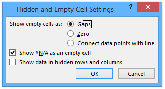
A new feature in Office 365 (and Excel 2019), Show #N/A As An Empty Cell, solves the pain and frustration experienced by generations of Excel users trying to avoid plotting what look like apparently blank cells.

Read about it in Plot Blank Cells and #N/A in Excel Charts.

This new behavior in Excel makes this article’s workaround obsolete.

---

Constable Henry: Just a moment, sir. I know everyone in this neighborhood, but I’ve never seen your face before. Can you account for yourself?

Freddy: Yes, I am Dr. Frederick Fronkonsteen, newly arrived from America.

by The FrankensTeam

This guest post is from the E90E50 FrankensTeam, i.e., Roberto Mensa, Kris Szabó, and Gábor Madács. The team has done a great deal of work with Excel and its graphics, and they’ve shown how many types of “advanced” graphics can be accomplished right in Excel. Such FrankenCharts include heatmaps, treemaps, network diagrams, and a number of other creative displays. Oh, and they’re as crazy about the movie Young Frankenstein as they are about Excel.

While I was reading Jon’s work using VBA Approaches to Plotting Gaps in Excel Charts I started to think, because I felt there had to be another solution which was waiting to be discovered…

Jon provided two different VBA routines as a solution for the problem: one changes the chart series formatting, the other changes the underlying data. As he clarifies at the very beginning, the disadvantage of using VBA routine is that it must be re-run every time the data changes.

Some time ago I realized that it is possible to use union of ranges in chart series. You can do it by using the union reference operator in the SERIES formula of the chart or via named formula. (The union reference operator is the same as the formula separator character, which is a comma in US-English versions of Excel.) In the project where it came up it was not particularly interesting, so I just stored this fact in my mind.

Now, a few months later, thinking about the gap problem… Eureka!

The union of separate ranges could be a solution, especially if we can build it up using the UDF within a named formula!

I was very excited by this possibility, so I quickly put together some code and shared the idea with Jon, who suggested some modifications in the UDF. Then we did a lot of tests with Kris and Gábor and corrected the problems showed up while we tested the solution in different Excel versions.

Let us explain how it could work.

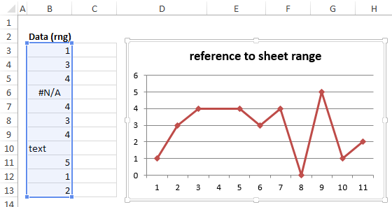
Below is a simple line chart plotting data from column B: the #N/A error value is not plotted (no marker) but the line is continuous, while the string is plotted as zero.

The series formula of the chart looks like:

=SERIES("ref to rng",,line_chart!$B$3:$B$13,1)

Where y values come from a continuous range: $B$3:$B$13

The idea

To plot gaps on the chart, you will need empty cells in the range used for y values. The union of ranges idea is very simple: we use the cells containing the number values from the original range (column B) but use empty cells from another column (column C) instead of the error or text values.

You can easily select the non-continuous range by mouse while holding the Ctrl key down.

On the below picture you can see how it looks from the Edit Series dialogue box.

And this is how the SERIES formula shows the union:

=SERIES("ref to rng",,
    (line_chart!$B$3:$B$5,line_chart!$C$6,line_chart!$B$7:$B$9,line_chart!$C$10,
    line_chart!$B$11:$B$13),1)

Note the y range is now surrounded by brackets, since it is composed of multiple areas.

You can easily define a named formula for the above range:

Name: y_rng_union
Refers to: =$B$3:$B$5,$C$6,$B$7:$B$9,$C$10,$B$11:$B$13

And use it as Series values:

Formula solution

To make a solution a bit more dynamic, instead of using static ranges, you can put together a dynamic solution with IF formulas. You have to check the cells one by one, and if the cell has a value to be plotted, then use the reference of the cell, else use an empty cell from another column. Then you separate the IF formulas by comma (or semicolon) to create the union of unique cells.

This way the chart will automatically be updated if the data changes, but if you have more data to be plotted, you will have to update the named formula manually.

For example you can put a similar formula to the name, supposing that column C is empty, so use the cells of this column:

Name: y_rng_union
Refers to: =IF(ISNUMBER($B$3),$B$3,$C$3), IF(ISNUMBER($B$4),$B$4,$C$4), IF(ISNUMBER($B$5),$B$5,$C$5), ..., IF(ISNUMBER($B$13),$B$13,$C$13)

Or you can use only one empty cell (for example C3) instead of the cells of column C:

Name: y_rng_union
Refers to: =IF(ISNUMBER($B$3),$B$3,$C$3), IF(ISNUMBER($B$4),$B$4,$C$3), IF(ISNUMBER($B$5),$B$5,$C$3), ..., IF(ISNUMBER($B$13),$B$13,$C$3)

More generally, you can use a name (for example x) referring to an empty cell:

Name: y_rng_union
Refers to: =IF(ISNUMBER($B$3),$B$3,x), IF(ISNUMBER($B$4),$B$4,x), IF(ISNUMBER($B$5),$B$5,x), ..., IF(ISNUMBER($B$13),$B$13,x)

If you are interested in the above formula solution, you may also find useful a help formula in an Excel range to build up the above (very long!) formula.

The logic is simple: A copy-down formula will concatenate together all the necessary IF(ISNUMBER(...) parts.

(Please note, if you use non-english versions of Excel, you will need to replace IF and ISNUMBER with your local language formula names. Also, you will have to replace the separator string (comma) if your version uses semicolons.)

For example, supposing that the header of your data is in B2, and data starts in B3, write this formula in cell M3 and copy down:

=IF(ROW(A1)=1,"=",M2&",")&"IF(ISNUMBER("&CELL("address",B3)&"),"
&CELL("address",B3)&",X)"

In our example we have to copy down this formula to cell M13 (since data ends in row 13). The string we get in M13 is exactly the formula we need to use in y_rng_union, so we copy M13 cell and paste as value. Now the formula could be copy-pasted as a reference into the name:

For better understanding, you can check these solutions in the without-udf example file.

Obviously the formula solution is not really effective and has limitations, but it could be an alternative for those who can not use VBA.

General solution with UDF-based named formula

For a more convenient resolution we will need some VBA code: a user defined function will build up the union-range and provide it to the chart, nested in a named formula. So if your data changes, the union range will change accordingly and if your data range grows, the chart will also capture new data.

Important to highlight that it will happen automatically, together with calculation, without any user interaction!

Here is the UDF code:

Function serie_with_empty(rDataIn As Range, _
        Optional cOffset As Long = 1)

    Dim rCellIn As Range
    Dim rCellOut As Range
    Dim rDataOut As Range

    Application.Volatile

    For Each rCellIn In rDataIn.Cells
        If Not IsNumeric(rCellIn.Value) Then
            Set rCellOut = rCellIn.Offset(, cOffset)
        Else
            Set rCellOut = rCellIn
        End If

        If rDataOut Is Nothing Then
            Set rDataOut = rCellOut
        Else
            Set rDataOut = Union(rDataOut, rCellOut)
        End If
    Next

    Set serie_with_empty = rDataOut

End Function

The procedure loops through the data range (first argument) and checks for non-numeric values. If the value is numeric (so to be plotted) then the cell itself is added to the union-range. If the value is not numeric, then another cell determined by offset will be added to the union. At the end, the function returns a range object.

This range object could not be used directly on the chart, it must be wrapped in a named formula.

To avoid errors when UDF could not be run (because macros are disabled) we suggest using an error check in the named formula:

Name: y_rng_union
Refers to: =IF(TYPE(serie_with_empty(rng,0))=16+NOW()*0 ,rng, serie_with_empty(rng,1) )

Where rng is the original data range, serie_with_empty(rng,1) is the UDF-calculated union-range.

The second argument of the UDF is the column offset parameter. Above we use 1 supposing that the column next to the original data is empty. You have to ensure a sufficient number of cells in this column. The offset parameter is optional with 1 as default value.

You can find more details about the logical test part of the IF formula under section Further details.

Using the above defined name on the chart, the result is correct with gaps, and refreshes as your data or underlying range changes.

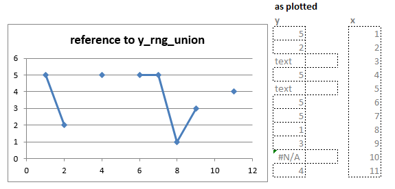
The method could be used for xy scatter charts too. For this chart type only the y values need to have empty cells for gaps, so no need to change the original x values range. As an example here is a possible SERIES formula of an xy chart:

=SERIES("ref to y_rng_union" , line_chart!$D$3:$D$13 ,
   Serie_with_empty_udf_xy.xlsm!y_rng_union , 1)

with the arguments:

x values (normal range): line_chart!$D$3:$D$13

y values (UDF calculations): Serie_with_empty_udf_xy.xlsm!y_rng_union

where line_chart is the name of the worksheet containing the x values, and Serie_with_empty_udf_xy.xlsm is the name of the workbook.

You need to reference the name y_rng_union to the worksheet or workbook. I usually start my chart with a regular range in the formula, so I leave the worksheet name and exclamation point intact, and replace the address with the named formula, like line_chart!y_rng_union. If necessary, Excel will change the worksheet name to the workbook name.

Below you can see what our example xy chart looks like, illustrated with ranges as plotted.

We created two example files, one for line chart, another for xy chart. We used random data, so after pushing F9 you can see how data, ranges and chart changes.

Further details

We need to test if the UDF was run or not.

In practice, macros are usually disabled in the Trust center under Excel Options. When you open the file, Excel will try to refresh the chart, but the UDF code will be unable to run, so the range will not be correctly built. The chart will raise an “Invalid reference” error message. Unfortunately, after enabling the macros, the chart will not be refreshed, because it remembers that the reference is invalid.

If the UDF can not run it results a #NAME error, which is number 16 in the TYPE formula. In this case the IF formula will give the original range, so the chart will get a valid range – although the line will not have gaps. To see the correct gaps, you need to enable macros and trigger calculation (so push F9). We use a volatile formula in the name ( NOW()*0 ) this is necessary for the chart to be updated after calculation. (The chart ignores the Application.Volatile in the UDF code!)

Problems with Cell.Text property

The base concept of gaps on the chart is to plot only numbers. In the UDF,

If Not IsNumeric(rCellIn.Value)

tests the cell’s .Value property. We were intending to provide another possibility for the users to mark unplottable data using formatting. For example they could set a custom formatting to hide 0 values if these should not be plotted. In VBA Cell.Text property could be used to get cell’s text as displayed on the screen, but using .Text property caused Excel crashes in case of xy charts. In case of line charts we have not observed crashes, but the SERIES formula was not visible on the formula bar, so we stopped using the .Text property.

About the authors:

Roberto Mensa, Kris Szabó, and Gábor Madács are three Excel-enthusiastics from Europe, thrilled to push the boundaries of Excel and do what seems to be impossible. You can find more about them on their team-site.