Excel has built-in chart types for clustered columns and bars, and for stacked columns and bars. One of the commonest charting questions in online Excel forums is, “How do I make a chart that is both clustered and stacked?”

This article demonstrates a protocol for building clustered-stacked column and bar charts in both modern versions of Excel, that is, Excel 2003 and earlier and Excel 2007 and later. The technique is a bit convoluted, and it requires an expanded data layout to get the appropriate appearance. And there’s an additional degree of complexity to get the category labels to line up neatly under or beside the clusters.
For those who need to produce many of these charts, and who don’t have 15 minutes to spend on each one, I have created the Peltier Tech Charts for Excel, a commercial Excel add-in that does the heavy lifting at the click of a button.

Built-In Column and Bar Charts
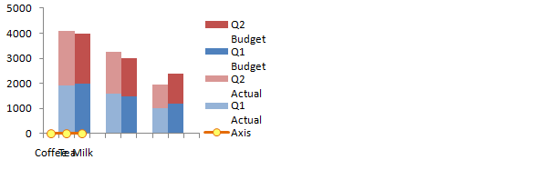
Let’s start with this simple data set, which compares budget and actual values for three commodities for two quarters of the year. We want to have clusters for each commodity, with stacked actual values next to stacked budget values within each cluster.

Without any effort or thought we can easily create clustered column or bar charts from this data.

Stacked column and bar charts are just as easy.

It’s not obvious how to combine the chart types. The protocol involves inserting blank rows and cells into the data range of a stacked column or bar chart, and values only appear in some of the places in the chart. The proper arrangement will cluster stacks of values with stacks of zeros separating the clusters.
Starting the Chart
I’ll leave the original data alone (always a good practice) and create a staging data region which is linked to the original data. The easiest way to do this is to copy the original data, then use Paste Special Link to start building the staging area. We’ll make our chart first, then explore how modifying the data layout changes the chart. In practice, we’ll modify the data first and then make the chart, knowing the effects of data layout on chart appearance.

The first step is to make a stacked column or bar chart from the data in B6:E9. There are no categories selected (i.e., the commodities are not part of the initial chart), so Excel just uses the counting numbers 1, 2, 3.

Since categories always start from the origin, the bar chart’s category labels go from the bottom up, instead of top down as in the sheet. So the vertical axis has to be formatted to make the categories go in reverse order. Also the value (horizontal) axis has to cross at the maximum category, which is at the bottom now, since the order of categories was reversed.

Adjusting the Data
So that’s only stacked. Let’s adjust the data by inserting some rows.

The stacks of columns/bars are now spread out. Not yet what we want.

But lets stagger the budget data by a row, to move the budget data points off the actual data and onto blank slots in the chart.

Unfortunately the staggering doesn’t happen automatically, so we have to go back and tell Excel what data range to use for the chart. Right click on the chart, then select Select Data or Source Data (the command is version-specific). Click in the Chart Data Range box, and select this whole data range.

One more adjustment to the data. Let’s insert a row at the beginning and end so there’s a space outside of the first and last cluster.

Again, we have to explicitly tell the chart about the updated data range. This is almost what we want.

Reduce the gap between columns/bars to give the chart a clustered appearance: select one series of columns, press Ctrl+1 (numeral one) to open the formatting dialog, and in the first screen you see (“Series Options”) change the entry for Gap Width to zero. Color code the data series to make it clearer which data series are associated.

In practice, it is not necessary to create a chart using the compact data and adjust it after every modification to the data. The correct protocol is to adjust the data, and then make the chart shown here, and proceed with adding labels, below.
Adding the Labels
Almost done. We need to add the category (cluster) labels. We’ll do this by adding a “dummy” series to the secondary axis, and the secondary axis will have the category labels we want. Add a column to the original data range for the dummy axis series (column F in our example).

Select this added data (F1:F4), and hold Ctrl while selecting the column with our labels (A1:A4), so that both areas are highlighted. Make sure you include the blank top cell in the first column. Copy the range, select the chart, and use paste special (Home tab of the ribbon > Paste dropdown > Paste Special) to add this data to the chart as a new series, in columns, with series name in the first row and category labels in the first column. In other words, use these settings:

In Excel 2003 and earlier, the original labels (1, 2, 3, etc.) remain along the axis, but in 2007, the new labels take their place, even if we hadn’t checked “Replace Existing Categories”.

Since zero value bars have zero height or width, they don’t appear in the chart. Just to show where this new series is added, I’ve temporarily replaced the zeroes in column F with values of 500. The series spans only the first three categories.

If you’re making a stacked-clustered column chart, convert this new series to a line chart type. Sometimes Excel 2007 doesn’t expand the legend enough to show the legend entry for Axis, so I’ve stretched it in this chart.
Manipulating the Axes
Now format the Axis series to place it onto the secondary axis. To do this, select the Axis series. If you can’t see the Axis series, click the dropdown in the top left of the Chart Tools > Layout or Format tab, and choose the Axis series. Then press Ctrl+1 (numeral one) to open the Format Series dialog. On the first tab, choose Secondary Axis.

Now add the secondary category axis, which is secondary horizontal in 2007 column charts and secondary vertical in 2007 bar charts. This command in on the Chart Tools > Layout tab.

We need to reverse the bar chart’s secondary vertical axis (like we did the primary when we first made the bar chart), and at the same time, make the horizontal axis cross in the automatic position, which generally means at zero or at the minimum.

Now we have to switch the position of the category labels. In the column chart, format the left hand vertical axis so the horizontal axis cross at the maximum, and format the right hand vertical axis so the horizontal axis crosses at the automatic (minimum) position.
In the bar chart, format the bottom horizontal axis so the vertical axis cross at the maximum, and format the top horizontal axis so the vertical axis crosses at the automatic (minimum) position.

Important – Axis Label Alignment
We want only half a slot on the outside of the first and last clusters, not the full slot shown above, to center each cluster on the commodity category labels. Format the top horizontal axis of the column chart, or the right vertical axis of the bar chart, so the crossing axis is positioned on tick marks. The bottom horizontal axis or the left vertical axis of the chart, which contains the labels we just worked so hard to add, should have the crossing axis positioned between tick marks.

Select the secondary value axis, which is scaled from 0 to 1 (the right vertical axis of the column chart, or the top horizontal axis of the bar chart), and delete it.
Format the primary category axis, which is scaled from 1 to 10 (the top horizontal axis of the column chart, or the right vertical axis of the bar chart), and format it so it has no tick marks or tick labels, and no line type.

Finally, select the Axis legend entry. In Excel 2003 be sure to select the text label, not the legend key (the marker and line). Press Delete. In the column chart, format the Axis series to be invisible (no marker, no line).

That wasn’t so hard, was it? Though it did take a very long time.
Adding a Line to a Clustered-Stacked Column Chart
It’s relatively easy to overlay a line chart series onto the clustered-stacked column chart. Instead of the column of zeros we used to generate our commodity axis labels, put in the values you want to plot, and add a meaningful column header.

When you go through the process above to add your labels and manipulate the axes, you will end up with data points where you want them. Just don’t bother hiding the series at the end of the process. If you want to show the line on a secondary axis, despite my warnings to the contrary, don’t delete the axis, simply scale it appropriately to your data.

Adding a line to a cluster-stack bar chart is much more complicated, so I will not cover it here.
Clustered-Stacked Charts in Peltier Tech Charts for Excel

This tutorial shows how to create Clustered-Stacked Charts, including the specialized data layout needed, and the detailed combination of chart series and chart types required. This manual process takes time, is prone to error, and becomes tedious.
I have created Peltier Tech Charts for Excel to create Clustered-Stacked Charts (and many other custom charts) automatically from raw data. This utility, a standard Excel add-in, lays out data in the required layout, then constructs a chart with the right combination of chart types. Charts can be made using data in a wide variety of arrangements, in either vertical or horizontal orientation.

This is a commercial product, tested on thousands of machines in a wide variety of configurations, Windows and Mac, which saves time and aggravation.
Please visit the Peltier Tech Charts for Excel page for more information.


Heather Ruddy says
Did you change the instructions for the clustered and stacked column chart from last week? I made several charts succesfully using the older version instructions but this update has me totally confussed!
Jon Peltier says
Heather – The changes are minor, and overall, I think this protocol is easier.
Heather Ruddy says
I guess I dont’ handle change well! ;) and I am having troubles replicating my charts – would it be possible to send me the old instructions via email?
Nina says
Thanks Jon. This is very cool. I actually do this using pivot table and chart it. However, I was wondering if you can cluster ‘actual’ stacked bars side by side and then the ‘budget’ stacks side by side, instead of coffee actual and budget together.
Donna says
I have a bar graph with 4 bars of data but one of the bars keep overlapping with another and I don’t know how to set it so they all sit next to each other, please help!
Donna says
Sorry – forgot to mention, there is a scale on either side.
Jon Peltier says
Hi Donna –
Sounds like your series are not all on the primary axis. The one(s) on the secondary axis are in front of those on the primary axis.
Is this a general question, or have you gotten stuck using these instructions?
Jon Peltier says
Hi Nina –
I think what you want to do is transpose your data (switch rows and columns) and then follow the procedure to modify the data and create the chart.
RD says
For the column chart, how do you switch the primary horizontal axis to be on top (1,2,3,4…10) to make the secondary horizontal axis (Coffee, Tea, Milk) to be on the bottom.
Nina says
Thanks Jon, I figured out a different way coz I am using pivot table and chart. I separated the data into two columns and plugged in zeroes in the blanks and grouped the variables in rows.
Your website is very helpful. I have learnt a lot about macros, add-ins and coding from your website. Thank you so much.
Taneeco Evans says
Jon:
Is it possible to create bar chart (100% stacked bar) with a secondary x-axis (horizontal)? I would like to chart percentage totals for multiple products, across more than one year.
I can create a 100% stacked bar chart with percentage on the x-axis and years on the y-axis. As I add years the chart gets taller. I would like for years to move horizontally. So, 100% product mix move across horizontally by year.
Thank you.
Donna says
Sorry – this is a general question. When I put them all on the primary axis, my scale on the right hand side disappears.
Roy says
Thanks for the instructions. It was a little confusing at first for me because my data was transposed from your example.
I tried inserting blank columns instead of rows, but Excel 2007 did not handle that the same way. So, I transposed my data and your procedure worked like a charm.
Would be helpful to see the Series Values as things progress.
In my original clustered chart, I had a line chart on the secondary axis. Changing to a clustered stacked chart really did a number on that. Once I finally realized that it WAS drawing the line, but since I had only 1 entry point every 5th cluster, I was not getting a line. Added Data Labels to see where the line would have been, then added Markers so I could have a visual of the line.
All-in-al, very helpful. I learned a lot about how Excel does clustering.
Lepski says
In Excel 2003 I am not able to go from the first picture to the second picture in section ‘Manipulating the axis’, because when I add a second category x-axis (after adding the second y-axis) this wil not result in a stretching of the line graph and thus the newly added categories stop short, i.e. I cannot align properly later on with the original x-axis. Am I doing someting wrong?
Lisa says
I am using Excel 2010. Trying to make a graph with horizontal bars.
When I try and insert the ‘dummy’ series, I can’t use the ‘Paste Special’ function as it doesn’t seem to exist. If I set it up as another series the only way I can use the category values is to replace the x-axis labels.
I tried using the dummy values then initially converting to a line, then the idea was to put it on a secondary axis then add labels. Once I change the format of the data series to line, it automatically sets up a a secondary y-axis but no x-axis, and the option of secondary axis for this data series is greyed out.
I am going round in circles, maybe someone can help??
Jon Peltier says
Lisa –
What version of Excel? To Paste Special, first copy the range, then select the chart. In 2003 & earlier, go to Edit menu > Paste Special. In 2007 and later, on the Home tab of the ribbon, click the down arrow on the Paste button, and click Paste Special.
Jon Peltier says
Roy –
“I had only 1 entry point every 5th cluster”
Go to the source data dialog, click on hidden and empty cells, and choose the interpolate option for empty cells. This will draw the lines to connect the markers across the gaps caused by the empty cells.
Donna says
Thanks so much!!!
I’ve been trying to make a time line graph for planned and actual dates for each project. I’ve been working on it for ever to try and have both clustered AND stacked bars….
you saved the day, and in such an elegant and simple way to the one’s I tried before I found this site (secondary axis, graph on graph etc.)
THANKS!
Wade Stevenson says
THANK YOU so much for sharing how to do this. You’re instructions are AWESOME!!! I have been trying to do this for some time and finally found some much needed help!
You ROCK!
susie says
i was able to do the graph, however, when i adjusted such that there will be no gap, the graph indeed removed all the gaps, including the supposed to be gaps between each category. what do i do with this?
thank you!
Jon Peltier says
Susie –
Do you have blank rows in the adjusted data, between data for the clusters?
susie says
i see. i wasn’t able to add blank rows on the adjusted data.
thank you very much! it worked perfectly now! your articles really helps a lot ;p
Alok says
There is a much more simpler way of producing such a chart in Excel.
Put your data in the format below:
Group A Group B Group C
Level 1 Level 1.1 5 5 5
Level 1.2 5 5 5
Level 2 Level 2.1 5 5 5
Level 2.2 5 5 5
Level 3 Level 3.1 5 5 5
Level 3.2 5 5 5
The Level 1,2,3 are merged cells. Level 1 is merged across level 1.1 and level 1.2
Select this entire data set and press the graph button in excel. Select clustered chart and see the magic.
Jon Peltier says
Alok –
I’ve taken a screen shot of the data to clarify it for other readers. I will note a few things:
1. I think you meant to choose a stacked chart. The top chart below is clustered, the bottom one is stacked.
2. Merging the cells makes no difference; Excel centers the outer labels across the inner labels regardless.
3. This groups the stacked columns using lines among the axis labels. This is fine in some cases, and I’ve written about it in the past (see for example Chart with a Dual Category Axis). But it has issues:
a. There are excess lines among the axis labels, which may make the chart seem cluttered.
b. There is an extra level of labels which may not be needed and may in fact add to the clutter.
4. You don’t get the visual clustering as in the tutorial above. Sure, you can reduce the gap width, add blank rows in the data (but make sure the cells highlighted yellow contain a space character to preserve spacing of axis labels).
But this does not solve the cluttered axis issues in point 3.
D says
Jon,
Thank you so much for this information. I still struggled with it a lot and spent a couple of hours manipulating the chart and data to get it to look right for my purpose, but your instructions made all the difference in the world! A million times thank you!
DB
Kate says
Jon,
Thanks for a super-helpful tutorial! However, I’m stuck on the “add the secondary category axis” step – are you able to tell me how to do this bit? I have added the “axis” series, and displayed on secondary axis, but this is a secondary vertical axis (mine is a column chart). Your next step says “which is secondary horizontal in 2007 column charts” – this is the bit I’m stumped on.
Thanks,
Kate
Brent says
Jon
Thanks for your efforts. Is it feasible to apply clustered columns with a Broken Y Axis?
Regards
Brent
Anonymous says
I’m also stuck on the “add the secondary category axis” step.
Gissell Dow says
Thank you so much! This helped me do EXACTLY what I needed to do.
Karen Driscoll says
I was tearing my hair out when I found this.
Great help.
Thank you.
Darren says
Hi, I’ve followed this (up the line bit, I don’t need a line) successfully, however as I have more data than you (weeks of the year, 31-52) I can notice that the bars start to visibly converge with the right hand tick mark on the Category Axis around the 6th week.
So you have any idea what, if anything, I can do to stop this?
Darren says
Ignore my last comment, just needed to include another row of data in my source data and now they’re all nice and tidy.
Darren says
For those struggling adding the secondary X axis, I had the same problem, see http://www.andypope.info/tips/tip008.htm that’s what helped me.
Melissa says
I have the blank spaces in and there are gaps between the bars but there’s still a blank legend for the gap that I can’t get rid of. If I delete it in the legend entries the gap goes away. Help please.
Eddie says
Hi Jon,
Is it possible to graph the double-stacked bars (primary y-axis0 on the same chart as a line (secondary y-axis)?
Jon Peltier says
Melissa –
You must still be using Excel 2003.
Click once to select the legend, then click again on the text of the label you want to remove., not just on the little square in front of the label. Then press Delete.
Jon Peltier says
Eddie –
The protocol uses a line chart series on the secondary axis to provide the axis labels. If you want a line series to put a marker where each stack in a cluster is, rather than centered on each cluster, you need to add a new series, move it to the primary axis, and make sure it’s a line series. Don’t mess with the line series that’s holding the axis labels in place.
The data would be arranged like this, based on the last worksheet screenshot of the post (before the comments):
Series Name: Cell F6
Data for Markers: Cells F8, F9, F11, F12, F14, F15
Blanks which are still part of series Y values: Cells F7, F10, F13, F16.
rebekah ann stoutenburg says
First, thanks for the amazing tutorial! I’ve actually enjoyed work this week because I’m learning. I am, however, stuck when trying to add a line to a clustered-stacked column chart. My data points (retail units in thousands) show up but I can’t get the connecting line to as well. Any idea? I was able to follow your instuctions until it’s time to manipulate the axes. Adding images of cell data along teh way would be helpful. I can’t tell if you’re actually typing “coffee, tea, milk” and “last year” into the ‘active’ cells B6:E16 or not. If you are, how and where?
Jon Peltier says
Rebekah –
Coffee, Tea, Milk are in A2:A4, and Last Year’s label and values are in F1:F4, as shown. I simply used these values instead of zeros, and unhid the markers and line so the points would appear.
rebekah ann stoutenburg says
Thanks, Jon. I didn’t understand your reply so perhaps I’m not asking the question correctly. I wish I could share an image so you could see what I mean, but I can’t from a work laptop. At this point, I’m stuck because I have coffee, tea, and milk on both the top and bottom horizontal axes. No clue how yours became 1-10! It doesn’t look like anything happens when I click on secondary horizontal axis from left to right. ??? (Excel 2007, column chart)
If we can directly email, please let me know!
Corwin Bennett says
Jon,
I am not able to convert just the axis part to a line graph. Can you please tell me how to do that part of the instructions? If possible a screen shot would help a ton.
Thank you,
Corwin
Jon Peltier says
Corwin –
I’ve enhanced the instructions for this part:
Select the Axis series. If you can’t see the Axis series, click the dropdown in the top left of the Chart Tools > Layout or Format tab, and choose the Axis series. Then press Ctrl+1 (numeral one) to open the Format Series dialog. On the first tab, choose Secondary Axis.
Jon Peltier says
Rebekah –
The beverage labels typically appear when you add the axis label series. They disappear when you move the axis label series to the secondary axis, and the original axis labels come back. The beverage labels reappear on the secondary horizontal axis (secondary vertical axis if it’s the bar version you’re making) when that axis is added to the chart.
Heath Mayer says
Thank you, thank you, thank you!! These instructions are awesome.
Dipanwita says
Hello Jon,
I have been struggling to get a basic chart with excel 2007. It was much much easier with 2003.
I have a table as below.
Step1 Step2 Step3 Step4 Step5 Step6 Step7 Step8
Rel 1 1′ 1′ 1′ 3′ 2′ 2′ 1′ 1′
Rel 2 1′ 1′ 1′ 1′ 2′ 1′ 3′ 3′
Rel 3 1′ 2′ 3′ 3′ 2′ 1′ 1′ 2′
Rel 4 1′ 1′ 1′ 2′ 2′ 2′ 3′ 3′
Rel 5 1′ 1′ 1′ 2′ 2′ 3′ 3′ 3′
Legend 1′ Done
2′ Not Done
3′ NA
Rel stands for releases and multiple releases are being worked upon in parallel.
I have to show the progress status of each release of the program in the form of a stacked column chart.
So basically, I need the releases in the x-axis, the steps in the y-axis, and equal length columns with 8 divisions, represented by 3 colors – done, not done or not applicable.
I am just not able to get the Steps 1 to 8 in the y axis.
Can you please help?
Dipanwita says
Oops…I do not think the cut and paste of the table came our well.
Basically each release has 8 steps and people are working parallely on multiple release.
So each release has some steps completed, some not completed and some not applicable.
In order to show status of each release w.r.t to the 8 steps, I need to have a stacked column chart. We can represent done, not done and not applicable step by different colors but each step needs to be of same dimension in the chart.
Cedric says
John,
I have followed your workflow and everything works correctly with your sample data however when I input my data namely a dates for secondary X axis it starts acting weird. The dates I use 7/1/2011 and 7/4/2011 and 7/11/2011. I place the dates where you have coffee milk and tea. When I get to secondary chart and expand it out it doesn’t expand out with those three dates it does a range from 7/1/2011 to 7/11/2011.
Cedric says
Jon, Sorry I misspelled your name the first time and accidentally hit send before I finished.
I have followed your workflow and everything works correctly with your sample data however when I input my data namely a dates for secondary X axis it starts acting weird. The dates I use 7/1/2011 and 7/4/2011 and 7/11/2011. I place the dates where you have coffee milk and tea. When I get to secondary chart and expand it out it doesn’t expand out with those three dates it does a range from 7/1/2011 to 7/11/2011 in integrals of 1. Is there a way to make sure it applies my dates?
Jon Peltier says
Cedric –
Excel recognizes your dates as dates, and tries to fit them on a date-style category axis. Select the axis, open the formatting dialog (Ctrl+1 is a handy shortcut), and on the main screen of the dialog, under Axis Type, change Automatic or Date to Text.
KR says
Hi. Thanks–very helpful. One remaining question: If I want to order the way my bars are stacked, can I do it? I’ve tried rearranging the data columns, but that hasn’t worked. I’m trying to use the stacked bars to model heights, and I want a particular column to be at the top of my stack.
Jon Peltier says
KR –
Without special measures, all stacks have the series in the same order. To make one column sit at the top, it has to have the largest plot order of all the columns. Change the plot order by changing the last argument of the SERIES formula, or by rearranging them in the Select Data dialog, by selecting a series in the list and pressing the up or down buttons above the list of series.
Patty says
My boss wants me to create a chart for him, and I don’t know if it’s possible. He wants a combination of unstacked and stacked columns. The first column would be the total college enrollment. The stacked column (next to the first column) would be broken into Outreach enrollment numbers for the various Outreach programs. By putting the college enrollment and the Outreach enrollment side-by-side, he hopes to show what percentage of total enrollment is occupied by the Outreach programs.
I hope I explained this in a way that you can understand. I would appreciate any suggestions.
Jon Peltier says
Hi Patty –
This is not difficult to do, by following this protocol. Your data needs to be all in columns, one column for Total College Enrollment, then one column each for all of the Outreach programs.
If you see my expanded data, Q1 and Q2 Actuals are in one row, Q1 and Q2 Budget are in the next, then there’s a blank row, and this pattern repeats. In your data, Total College Enrollment goes in its own row, then all of the Outreach are in the next row, then a blank row, repeating as needed.
Lauren Womack says
John, this is so great, I can ALMOST see it doing what I need to do.
But, before I can plug my own, real data into your ‘template’, I need ot get past:
“We need to reverse the bar chart’s secondary vertical axis (like we did the primary when we first made the bar chart), and at the same time, make the horizontal axis cross in the automatic position, which generally means at zero or at the minimum.”
For the love of me, I have no idea what this means, and I am flat-out stuck.
Can you help a sister out?
Thank you.
Lauren Womack says
Forget my previous question – I finally got around it.
I do have a follow up question to Jon, or anyone else using this method.
Is there a max number of data points you can use?
As I see it, the sample has 3 – Product, Quarter, Actual.
Could you do it with 4? Say, site, job gain, job loss, month?
I can’t see a way, yet, and I wonder if that’s because there isn’t?
Jon Peltier says
Lauren –
This approach breaks the data among three factors. There is no clear way to break it down further. What you would have to do is either combine one factor (e.g., lump all quarters together to get a total) or make separate charts to show each factor (one chart for each quarter).
Scott says
Jon:
I cannot get the Q1 Budget and Q2 Budget to move to the “2” column. I understand that i have to right click the chart and click “Select Data Source” (excel 2007), however, I don’t know what to do from there? I’ve tried a number of thing to no avail. What am I missing in your instructions?
Thanks
Jon Peltier says
Scott –
Have you offset the budget values down one row from the actual values?
Scott says
Yes. I recreated your spreadsheet and I inserted the extra rows and moved the Q1 and Q2 budgets down one row.
Scott says
I’m not able to convert my “print screen” image to a picture for you to link to help us out.
Scott says
Jon,
Good news! I figured it out. So, I have a suggestion. Edit or add this to the following:
“Unfortunately the staggering doesn’t happen automatically, so we have to go back and tell Excel what data range to use for the chart. Right click on the chart, and select Select Data or Source Data (the command is version-specific)….
… When the “Select Data Source” window pops up, click in “Chart data range” and select your entire chart data again.
Thanks for being willing to help. I may have another question. LOL!
Scott
Kris Thurman says
Great post. Everything worked like a charm until I get to:
“We want only half a slot on the outside of the first and last clusters, not the full slot shown above, to center each cluster on the commodity category labels. Format the top horizontal axis of the column chart, or the right vertical axis of the bar chart, so the crossing axis is positioned between tick marks.”
I totally get what the purpose is, but in Excel 2003 I can’t figure out how to do this. Could you possibly tell me ste-by-step how this can be done in Excel 2003?
Thanks!
Jon Peltier says
Kris –
Select the axis, press Ctrl+1 (numeral one) to open the Format Axis dialog, and where you edit the scale of the axis (first view in 2007+ or Scale tab in 2003-), check the option whose labels indicate “crosses between”.
Kris Thurman says
That worked perfectly. I tried that multiple times before and now I realize that I needed to DESELECT that option – Duh. Thanks for your help!!
Maheswaran says
Hi Jon,
I have a requirement to draw clustered Stack chat with the following information,
Products Total Spent Forcast
A 10 6 4
B 14 10 2
C 2 4 3
Spent and Forcast should be in stacked with total in clustered. How can I achieve with excel 2007?
Maheswaran says
Hi Jon,
After going through this post I was able plot my chart on my requirement mentioned in comment :).
Thank you very much for this post.
-Mahesh
Austin says
I just want you to know what a great help your website has been to me over the past few years. Tips like this have solved SO MANY of my frustrations with excel when I know what I want something to look like but don’t know how to create it. A MILLION THANKS!
John says
Your tips were great and I was able to create the graph I wanted, but now I need to insert error bars and it is not working. I can only get excel to add error bar and I have 5 pairs of bars. I have made tons of figures and know how to use the custom function. Have you had issue with error bars and stacked figures? Any ideas on how to fix it.
Thanks.
5.antiago says
This was excellent, thanks. Your grasp of every detail in Excel never fails to impress!
Jose says
Very helpful, although I can’t seem to center my axis labels between two stacked columns. I lines up directly under one column. I know it has to do something with the “summy” series, but I can’t seem to figure it out. By the way, I am using Excel 2007
psalm268 says
Hi, I can’t figure out what you mean by paste special under the adding the labels section. And i also can’t get the category labels and the axis line to spread to the rest of my chart. They stay under the first set of clustered/stacked columns. Would you be able to help me out? Thank you.
Otherwise, this seems to be the data I’m looking for, as I am seeking to have clustered, stacked columns and then add a line on it to show percentage trend.
Jon Peltier says
After you copy the data, select the chart, and from the Home tab, click on the down arrow thingy at the bottom of the Paste button (or in 2003, choose Edit > Paste Special) and select Paste Special.
Then follow the instructions carefully to make sure you move the label series to the secondary axis, add the secondary horizontal axis, then make sure to format the primary horizontal axis crosses setting is set to “between tick marks”.
Amber Davis says
Thanks for this article! It helped me a lot.
psalm268 says
Thanks! It worked!
This is a great article. Kudos!
Asanwa says
Hi Jon
I need to create a bar chart for my boss with the following sample data. I have created my secondary axis (% identity) which is on the right. However the numbers on the primary axis comes up twice!! Please can you help as I don’t know what am doing wrong. Thanks!
Identity No.Identity % Identity
Identity 1 3 2 65%
Identity 2 0 0 0%
Identity 3 0 0 0%
Identity 4 0 0%
Identity 5 2 0 50%
Identity 6 1 2 100%
Identity 7 2 0 50%
Identity 8 2 0 50%
Identity 9 2 0 0%
Identity 10 0 0 0%
Jon Peltier says
Asanwa –
I don’t know how you are plotting this data, or how it relates to this chart type.
Daphne says
Thanks for the help!! This was really useful..
How do I get rid of the gaps between columns/bars to give the chart a clustered appearance though??
Thanks!
Jon Peltier says
Daphne –
Select one of the columns, press Ctrl+1 (numeral one) to format it, and on the main view (Excel 2007/2010) or on the Options tab (Excel 2003/2002/2000/97), change the gap width to zero.
shal says
Thanks a million for writing on graphs.
I tried doing you way, however, i cant reduce the gap for each two just like yours. every column of mine has space in between. hope you can clarify.thanx!
Kevin says
Very instructive! I want do something even more complex: Expenses by category and subcategory, with the clustered columns representing the categories and the stacks representing the subcategories. Here’s the complication: the subcategories change for each category. For example, category Activities has subcategories Soccer, Baseball, Hiking, etc.;
category Charitable Donations has subcategories American Heart Assn, American Red Cross, Habitat for Humanity, etc.; category Dining Out has subcategories Pizza, Fast Food, Salads-Sandwiches, etc. In a perfect world I’d be able to put data labels on each segment of a stack.
I can do this easily with separate charts for each category and its subcategories, but one huge chart is the holy grail. Is this possible without spending hours?
Kinn says
You are AWESOME! Thank you so much for this development. You made me look like a genius :-)
Bryan says
Great tool, it worked perfect on the stcked columns but I need lines in my graph. How can I leave the lines without them being distorted. I tried smoothing the numbers out across each cell the lines are reading but it still is very wavy. Any help would be appreciated.
Thanks,
Bryan
Jerred says
is there an excel example that can be downloaded for the clustered bar chart?
Jon Peltier says
Bryan –
What kind of lines? And how are you smoothing the numbers (I don’t know what you mean)?
esperluette says
Thank you!
Jon Peltier says
Bryan followed up:
When I insert new columns to allow for the clustering it cancels out my
lines because it has rows that do not have data in them. I have to add
data to the columns that were inserted to allow the lines to show up.
The smoothing I am talking about is averaging the numbers in the new
columns, i.e. if I have 1000 and 2000 between two columns and have to
add 2 columns to create the new the stacked cluster then I have to fill
in data into the two blank columns added 1000, 1333, 1666, 2000 but
when the graph reads the line it is extremely wavy.
My response:
Right click the chart, choose the option to adjust the data, and click the Hidden and Empty Cells in the bottom left of the dialog. Choose the option to draw a line across the gap. This means you won’t have to manually interpolate the line across the gap.
Lea says
Hi, I am fairly new to graphs using 2007. I know how to create a gap between each bar, BUT, how do I change the width of the bars themselves????? They come our really skinny and hard to see.
Thanks, Lea.
Jon Peltier says
Hi Lea –
If you have set Gap Width to zero, but the bars are still thin and far apart, it’s probably because you have dates on the category axis. So for example, if you have one value each week, the bar will be as wide as one day, and there will be six blank spaces between the bar and the next bar. Change the axis type to text instead of date or automatic.
Joy says
Thanks very much Peltier! I m wondering if you can make the charts in 3 D with Excel 2003 this way?
Jon Peltier says
Joy –
3D charts limit the ways you can combine chart types and secondary axes. Which is a good thing, because they also are an ineffective way to try to display data.
Alex G says
Hi,
Is there a way to add a clustered column to the 2 already existing stacked columns?
Thanks!
Jon Peltier says
Alex –
Sure, but what you need to do is add them to the expanded data. Keep in mind that a “clustered” column in this case is simply a stacked column with only one in the stack.
The first example shows how you might add another category (Soda) that has a total that’s not broken into Q1 and Q2. The second shows how you might add a third item (Benchmark) that’s not split into Q1 and Q2 to each cluster of items that is split (Budget and Actual).
Reggee says
hello. is there a way to show on the same graph a single bar as well as a stacked bar. . . for example I want to show single bar total of 100 units, along side it I want to show out of that 100….70 units used and 30 remaining and show the 30 on top of the 70 to equal the 100 bar …hope that made sense . . thx
Ronald de Raaff says
Hi Jon, Did you describe anywhere a methode of having a vertical line (based on percentage data) on a horizontal stacked (100%) bar chart?
Thxs Ronald
BTRabbit says
This is awesome and it works perfectly for me… wow…. what a smart person
thanks
Jon Peltier says
Reggee –
Check the comment right above yours. A single bar clustered next to a stack of bars is really just a stack of 1. Sounds like you want to use the single bar like a benchmark (or target), use the second example.
Naomi Oyemwense says
Jon,
Hi! It is 7:43 p.m., and I am so stuck!!! I am using excel 2003, and I have used a pivot table in order to create a stacked graph. I’m not sure how to include “space characters” in my raw data in order to add additional spaces/separators in my graph. Basically, I’m trying to make a stacked graph into a stacked and clustered graph by adding in blank spaces. Is there anyway that I can do this?
Thanks,
Naomi
Jon Peltier says
Hi Naomi –
Unfortunately you can’t use a pivot table directly in this technique, nor can you turn a pivot chart into a clustered-stacked chart.
What you can do is copy the pivot table, then paste special-link on a new sheet (so if the pivot data changes, this data will adapt). Then follow this technique to make your chart.
HansL says
Your example shows data on one axis representing dollars(budget). Is it possible to develop a clustered stacked chart whereby you might have dollars as one stacked column next to, say, a stacked column representing units sold with data data on a secondary vertical axis.
Jon Peltier says
Hans –
You could develop a chart that has some bars on the first axis and other bars on the second axis, but you’re asking for trouble. No matter how clever you are indicating which bars go with which axes, people will be confused.
It would be better to normalize the different classes of data, for example, % of target, or % of highest overall monthly value.
Ellen says
Jon,
I am stuck on my chart. It’s almost the way I want it, thanks to your tutorial, but not quite perfect yet. It seems the problem has to do with my “labels”, which are dates. I cannot get the labels to line up underneath the columns. And it would be really nice is the last label/date, 1/31/12, would display along the axis. Can you help?? Thanks in advance!
Here’s a picture of my chart and my data:
http://www.freeimagehosting.net/dob26
Tanu says
I want to know whether i can custom a label in column chart. i mean if my chart label is having 80000, 70000, 65000…. and i want a ratio which i have in another column to appear at the top of each bar where label appears. I simply mean cud i add another row or column as label??
David Lakeland says
Jon, do you have any tutorials that combine clustered columns with stacked graphs – or is that not possible? Thanks, DL.
Jon Peltier says
David –
If what you mean is, you want a single bar clustered next to a stacked bar, well, consider a single bar is a stack that is one bar tall.
Consider the data I started this exercise with. Confine yourself to columns A:D (delete or ignore column E), and construct the chart.
Cathryn Lambourne says
Hi Jon
Thanks for the details of how to build the stacked cluster chart. It worked well but I was having trouble with getting the category labels to line up properly on the x axis. In desperation I tried inserting them in my expanded data table in the first column. I merged the category label across the stacked expanded data for that category, then added it as a horizontal (category) axis in the ‘select data’ box and hey presto it inserted my category labels along the bottom.
I’m so pleased with myself I wanted to share it with you. Sorry if you had already come across this shortcut.
Greg says
Jon,
Thanks so much. I need to add a data table under this chart, is that possible?
Jon Peltier says
These in-chart data tables are usually more trouble than they’re worth, since you can’t omit some of the chart data nor apply much formatting. How about making a table in a range adjacent to the chart, and showing the range and chart together?
Jon says
Jon,
Thanks for another great tutorial. I’m stuck on trying to make what I thought was an easy change. I have one set of columns that contain three stacks and the neighboring column is one value. I have no problem making the graph as above with the three-stack on the left and the single-value column on the right. However, I’ve been trying and trying to switch them (single-value column on the left), but it doesn’t seem to want to stay there.
Any suggestions?
Thanks.
Abebew says
Hi Jon,
I want to thank you for your great contribution in my data analysis specialy for graphing.
I have one problem. How can I insert error bars on stacked clustered charts using 2007 excel.
Thanks
Vik says
I did all the steps and this works great. My only problem is the color coding. When I click on a bar to change the color, it doesn’t let me manually change the colors for every bar in a series at once but rather one at a time which would take forever.
In your example, this would be like needing to change the color on each of the Q1 Actual bar segments manually instead of being able to change them all at once. Is there a way around this? I have about 30 different bars so it would take a lot of time to do this. I am using Excel 2007. Thanks!
Jon Peltier says
Vik –
Each individual series (that is, each series which has a name in the legend) has to be formatted differently than every other individual series (that has a name in the legend). If you select one of these series, and use the paint can tool to fill the first series, you can then select each additional series and use the F4 function key to repeat this formatting on the new selection. Repeat with Select-F4 as needed.
John Niedermeier says
Is there an easy way to produce a stacked bar chart with counts of occurence on the y-axis and Fiscal Week (FW) on the x-axis? The problem is that most of the FW’s have no occurences, but I want all of the FW’s represented so that the data is spaced as they occur throughout the year. If it matters, I am trying to do it from a pivot table.
Jon Peltier says
John –
You can change a field’s settings to show items with no data. This would preserve the FWs with no occurrences, with blanks in the values field.
Adam Tomlinson says
Hi John,
This tutorial looks great and will do exactly what I need, but I have one problem that I cannot seem to resolve. When trying to add labels when I copy the 2 columns and then paste into my chart it comes up with amessage saying “Maximum number of series in a chart is 255” and it adds a whole lot of blank series??
Any thoughts as to what I could be doing wrong?
Many Thanks
Adam
Jon Peltier says
Adam –
Did you select the entire columns? Just select the two-column data range, and try again.
Adam Tomlinson says
Hi John,
The error seem to come when I selected the option for replace the series names, when I don’t it seems to work… Not sure why but happy it works now
Thanks again.
Jon Peltier says
Adam –
I’ve added a screen shot of the Paste Special dialog, so it’s clear what settings should be selected.
Z. Smith says
Regarding Error Bar not showing up issue:
I successfullly created the plot, and tried to put error bars on the columns, and the error bars wouldn’t show up. Originally the data for the error bars was coming from elsewhere in my sheet.
The FIX to get the error bars to show up was to organize the error bar data in a new column with rows matching the original data rows – i.e. data in A2 & A4, put the error bar data matching this data in say B2 & B4. Then select the whole range – i.e. data range =A1:A5, matching error bar range =B1:B5.
Hope that makes sense. Would be better with a picture, but I just don’t have time to generate one.
Jon Peltier says
Z –
Thanks for the clarification. I always find it less problematic if I put all of my data in adjacent ranges. I forget to mention this, because I take it for granted, but it’s not obvious to the typical user.
dwi says
Hi Jon,
this short tutorial is really helpful for me.
I am trying to make plan vs actual chart, the plan chart is consist 3 data which will be shown in stacked chart and then compared to actual in clustered.
thank you.
cheers
Vic G says
Hi Jon,
I’m new to VBA and Excel Macros.
I wanted to know whether what I need (listed below) is possible without invoking Macros. This is a project management tracker we are creating.
1.) I want to follow completion of 3 activities. A, B and C. and the status can be Red, Amber or Green depending on completion status.
2.) ‘A’ activity will be tracked for 50 cities in a stacked bar configuration, with each city status being Red, Amber or Green. Activities ‘B’ an d’C’ will also be tracked similarly (stacked) but all three are a cluster.
3.) The next cluster of 3 will be for a second province with a further 50 cities.
I hope this is clear. I just need to know whether this is possible without VB. If it is, I could use some pointers.
Silvia says
First of all, thank you again for the handy tutorial on this topic. Once I created the clustered column chart, how can I expand the range? In other words, I have the chart looking exactly how I want it now (I created it last year, following your tutorial), and want to add the last year.
If I ‘select data’ it tells me that the data is too complex to display, and if I select a new range it will overwrite everything – and if I do that, I get a complete mess.
It would be great if I did not need to redo all the formatting on the chart, just be able to add the last 4 quarters. Alternatively, if I know that it is not possible, I won’t spend any more time on it.
thx a lot!
Silvia says
Well, I just figured it out – it seems that posting on this board helped my inspiration :). I just had to go into each data series separately and change the range – selecting the whole range produced strange results.
Jon Peltier says
Silvia –
I like when smart people figure out the answers by themselves and then post it for everyone to see. Saves me the effort of saying the exact same thing.
One thing that might help is the small utility I discuss in How to Edit Series Formulas. If a bunch of series in the chart now end in row 6 and you need them to extend to row 10 (for example), the program lets you edit all series formulas at once to make this change.
Steve says
Jon…
When I try to add that blank row at the beginning and end of the data block to provide a little separation between the first column and the y axis and the last column and the right edge of the graph, (my equivalents of) the Q1 and Q2 Budget series “uncluster” and get stacked back on top of the Actual series. I don’t know if this matters, but I associated the Budget series with the secondary axis before attempting to insert those final blank rows.
While I’m “stuck” with the technical problem noted above, perhaps I’m headed down the wrong road anyhow. I see where you have advised against using a secondary axis for these types of charts because the user will have a hard time interpreting them. In my case, I’m wanting a chart that will show number of wildfires by year and number of acres burned by year, for a 10 year period, but further broken down (hence the stacked bars) by wildfires’ subclassification as either a “large” or “small” incident. Since acres burned per year typically sum to hundreds of thousands, while the count of fires is in the mere thousands, I had to associate the count of fires with the primary axis and the burned acres with the secondary axis. Your tutorial is helping me compose that chart. But… if you have a recommendation for a different style of chart to better convey this blend of information, I would appreciate your advice.
And, like so many others, I’d like to thank you for your excellent website, your technical expertise, and your willingness to share.
Silvia says
Jon – thanks for that reference, great article. For reference, part of my previous trouble with editing the series range was due exactly to the chart having been copied from a different file, which was even in a different directory (which is one of the cases you discuss in the article).
Thus, the path was very long, and the issue was that the arrows did not work in advancing the cursor, but introduced cell designations. The final workaround was to go directly and select the range I wanted, while the original series range was highlighted by default.
I will check out the utility you mention, and also dynamic charts – concept I hadn’t heard before.
Silvia says
Steve – Why do you want to present both the number of fires and acreage in the same graph? It seems too much, especially if you break down the fires by sizes.
Anyway – one work around would be to normalize your acreage to the number of fires, so you can use a single axis, and then include in the heading, or legend, or just a text box, the normalization factor.
In other words, let’s say you have 5,000 fires and 300,000 acres in year 1, you could scale the acreage by dividing to 60 all the acreage numbers. Then in year 1 the two bars will have equal height, and then in future years they’ll be similar in size, so you can use a single axis.
This way you are also conveying more information – and this in itself is a reason to have these two entities next to each other, rather than in separate graphs. Right away people could see that a rough order of magnitude for the average number of acres per fire was 60 in year 1 (in the example above). Also, they could get a feel for how did the problem evolve over the 10 years. Of course, you’d need to specify the normalization factor in the legend.
Adam says
Hi Jon-
Great instructions! I’m having one problem. I’m have showing data for 16 dates…each date includes 3 clusted bars, each stacked with 2 pieces of data. My bottom (secondary) axis contains the dates. After I complete everything, most of the dates are not aligned with the center bar of each cluster. The date on the far left is way to the left of the three bars. The date slightly “moves” to the right with each subsequent cluster. So it looks correct in the middle clusters. But then it looks too far to the right with the right clusters. Any thoughts?
Thanks!
Adam
Jon Peltier says
Adam –
First, make sure the axis with dates is formatted as a text axis (not a date axis or the default).
Then go up to the subheading that I’ve just inserted, “Important – Axis Label Alignment”, and check the positioning of the crossing axes.
Renee says
Hi Jon…I am trying to make a stacked bar chart..where there is only one bar for each month and then the month is divided up by categories (different colors)..
for example, I have 120 orders in the month of this 80 are on-time; 30 are late and 10 are shipped wrong..then I would like to be able to have this type of bar chart for the entire year..much the same as these categories and probably more ..
I am unsure how to format the data too..thanks so much for your help!
pao says
Thank you for your technique
Stefan says
Awesome how-to… quite a complex topic but it worked in first try! Thanks a lot!
Chuck says
Thanks for the great description! Worked well with Excel 2010
Jason says
Just wanted to say that this was an incredibly helpful find – thanks very much!
Charlotte Pijnenburg says
Hi there,
Thank you so much for this tutorial, it has helped me big time.
I just can’t figure out how to switch the the primary horizontal axis to be on top (1,2,3,4…10) to make the secondary horizontal axis (Coffee, Tea, Milk) to be on the bottom in Excel 2010.
I hope you can help me with this, I really don’t get how to do it.
It would be awesome if you can send me your answer by email.
Thank you so much!
Charlotte
Tania Maddigan says
Thanks for this fantastic information, which I used to create some wonderful graphs. Since setting this up, I have moved from Excel 2007 to Excel 2010 and the graphs no longer look so wonderful. Any suggestions on what I need to correct. Thanks in advance
James says
Thank you. I succeded.
Lostbutfound says
Thanks SO MUCH for this amazing information :) Definitely bookmarking your page for future reference! Really, thanks a million!
Rob says
The Paste Special in Office Mac looks very different and doesn’t have the options in the tutorial. Would you suggest any other approach?
Oak says
I’ll go against the steam here and say the instructions are poor. Especially the bit that says “Now add the secondary category axis, which is secondary horizontal in 2007 column charts and secondary vertical in 2007 bar charts”. The rest after that may also be rubbish, but that’s where I’m stuck anyhow
Jon Peltier says
Oak –
Thanks for the constructive criticism. I’ve reworded the section you had problems comprehending and indicated exactly the commands to use.
Amber says
hi Jon,
quick question – i have had success using your method as desribed. I was wondering if there were any trouble shooting points you could add if i am trying to do the same thing, but have some negative values included in my data set?
thanks, Amber
Amber says
Ps – much appreciate the post, made life a lot easier!
Jon Peltier says
Amber –
When you stack values, it’s very difficult to represent negative values. The top of the stack doesn’t represent the total, because the negative values have not been deducted. The total height of the stack is even more misleading because it includes the absolute value of the negative values. If the negatives are important to the analysis, you should consider alternative graph types.
Amber says
Hi Jon,
fair enough. What about if i only use negative data in isolation (i.e. not stacked -one column to itself) and then have stacked data in another column? e.g. have negative profit in one column by itself and then positive revenues and positive Cash flows stacked in the second column?
No worries if not possible, just thought i would ask.
thank you, amber
Jon Miller says
Hey Jon, thanks for the tutorial. I was painful at first but once I got through it, I’m finding it particularly useful. I used it to show various vendor product lifecycles and how our company aligns our internal adoption and support to the vendor. Having completed all of this, I’m left with one last desire: To add one extra line denoting the current date.
Alas, you mentioned that “Adding a line to a cluster-stack bar chart is much more complicated, so I will not cover it here.” Perhaps you could just give me a hint or an alternate tutorial that I could use to figure it out?
Thanks,
Jon Miller
Cullen says
Hi Jon,
I would like to know more on the header “Important – Axis Label Alignment”. It seems that i am unable to place the crossing axis positioned between tick marks. I have tried changing the number of categories between the tick marks but in vain. Could you share some light on my screenshot?
http://i48.tinypic.com/14d2b8w.jpg
Jon Peltier says
Cullen –
You have nine clusters in the chart, but only eight months on the axis. Extend the X and Y range for the axis series by one cell. Then format the top horizontal axis so the value axis crosses on (not between) tick marks.
Logan says
Hi,
I am trying to generate a cluster-stack chart where one stack uses one axis, and the other stack uses a secondary axis (scale issue — i.e. have large spend values by category, but small recoveries by these same spend categories). How can I accomplish this?
Thanks,
Logan
Denise says
I am stuck on the part that says to select F1:F4 while holding CTRL and select A1:A4 so both are highlighted. When I try to do that, Excel tells me “That command can not be used on multiples sections”. I am sooo close but I have no labels on the bottom axis. Any advice on what I am doing wrong?
Jon Peltier says
Select one of the ranges, hold Ctrl while selecting the other. Even if you don’t do this, the error you mention happens after another action, perhaps when you copy the range. If the two columnar ranges are not the same number of rows or don’t start in the same row, you will see that error.
Erin Corduan says
Thank you SO MUCH for this post! It is one of the best excel helps I’ve ever seen – so easy to follow and you’re explaining something so difficult! You rock.
Cameron says
Hi, thanks a ton for this guide. It worked perfectly. There were some points where I found it a little difficult to follow, but I think it’s mostly because of the new version of excel. Best regards!
Lenny Zimmermann says
Great stuff! Thank you for making it available.
I think this is the kind of chart I should be using for something I’m working on, but there are parts of it that I’m either not sure how to make it fit or where the date comes out very… asymmetrical. What I would like to be able to do is create a chart similar to the following: http://1.bp.blogspot.com/-Ch69snN2msk/T-ZEQZ4NhGI/AAAAAAAAB6U/NMK5uNdBkrg/s400/ChrMap623.jpg
I have data that looks like this:
Chromosome | Ancestor | Start | End
1 | (Length) | 1 | 100
1 | A | 1 | 30
1 | B | 20 | 40
1 | B | 70 | 90
2 | (Length) | 1 | 90
2 | B | 10 | 50
2 | B | 70 | 80
2 | C | 30 | 50
And so on. So it seems to me that the cluster here is the Chromosome number (22 clusters total in the real data) and the stacks would be a Reference Length or Ancestor name. The problem I have is how to reference the positioning information. I would need to see if I could get the chart to plot just a, say, gray line for the reference length for the first data segment in the cluster. For the second (1.A, if you will) I would need it to make a red bar from out to 30, then the problem child for B shows up where I would need something like a grey bar for 0-20, blue for 20-40, back to grey for 40-70 and then back to blue for 70-90. So the first subset (1.Length) only really has 1 data point, the second (1.A) has 2, and the third (1.B) has, essentially, 4 (assuming I have to work out all of the appropriate lengths.)
How do I represent that data when the columns for it are not symmetrical like all of the rest of the examples above? Or am I just looking at doing this completely the wrong way?
Sincerely,
Lenny Zimmermann
Jon Peltier says
Hi Lenny –
Looks like an interesting application.
You have 23 categories (22 plus X). What makes the data tricky is that you will need multiple data columns and chart series for the gray stretches, and also for the colored stretches. Probably it’s easiest if I build part of it for you. This table shows my eyeballed data for the first six chromosomes, normalized so the first chromosome is 100 units long. Notice the upper member of each pair has 11 columns and the lower member has 9.
When the data is spread out for charting, it looks like this.
And here’s the chart, with all the bars formatted appropriately.
Lenny Zimmermann says
Interesting…. I think I’ll need to look at that more closely to get my brain wrapped around it, but that sure looks right. Very awesome! I would note for most genetic genealogists it would still only be 22 since X is a bit… odd, to work on matching for genetic genealogy purposes, and the real values are a LOT bigger (chromosome 1 ends at 247,093,448, chromosome 2 at 242,697,433 and so on) but it shouldn’t be too many gaps for each data set at least, so I do have to figure out all of the differences to set the sizes of those gaps.Thanks!
Jon Peltier says
Larry –
I was just making up numbers based on inexact eyeball digitization. But whether the data is normalized to 100 or to 247,000,000, the approach is the same.
Olivier says
Hello Jon,
How do you do it when you want to use the clustered-stacked chart with the y axis that is on a log scale?
The closest data to the x axis disappear… It just shifts the next data up.
Could you please let me know how to sort this out?
Many thanks.
Cheers,
Olivier
Jon Peltier says
It makes no sense to use a log scale with a stacked chart. How are you going to compare the values of bars that are offset from each other?
Olivier says
Hello Jon,
I have realised it.
Is there then a practical way I can combine the clustered-stacked chart with your practical panel chart?
When selecting the data, Excel doesn’t display (keep) the range of existing cells but says that the whole range needs to be selected again with the new one.
It’s a bit dodgy…
Any idea please?
Many thanks.
Cheers,
Olivier
P.S.: Your website is tremendous.
Daniel says
This is brilliant, Jon. Thank you so much! My supervisor had given me a weird excel list to convert to a chart and I was struggling (typical Intern style), till I stumbled upon this instructions. Your comment about the merged axis to give it a cluttered X axis was exactly what I was looking for.
Bookmarked! :)
Regards,
Daniel
Swathi says
Hi Jon – This is great stuff and exactly what I was looking for. I could follow your steps and successful complete it. Further to this, I need to add % share each of the stacks. For example: Coffee Budget stack should show whats Q1 and Q2 % share on the bar, and Coffee Actual stack should show Q1 and Q2 % share on the bar. Is this possible?
Hannah says
Thank you so much, this is perfect. A mystery solved.
Alesha says
Hello Jon.
I am stuck at the point where you reverse the secondary vertical axis to get the labels from the top to the bottom. I was going great guns till then & now I’m going mad again.
Cheers.
Jon Peltier says
Alesha –
Are you unable to reverse the axis? What is the problem?
Alesha says
Sorry Jon, I wasn’t very clear was I? I sent you an email but just in case you didn’t receive it…
Under the section ‘Manipulating the Axes’ – I cannot find how to reverse the secondary axis on MS10. When I started with just the primary it was as simple as clicking select data & then clicking the box that says ‘switch row/column’. But since adding the secondary axis that option is greyed out. Until I work out this bit I can move on to the labels and finish the task.
Cheers.
BarryK says
Very helpful! Took me a while to figure out how to set the “X” axis to “TEXT” but once I fixed that, the result was beautiful!
Harihar says
In the above stacked column and bar chart you have showed coffee,tea & milk in different bars but Q1 actual and Q1 budget in single bar. If i want to for coffee in single bar Q1 actual or three month individual actual and below actual a single bar presenting Q1 budgeted or three month individual budget. same for tea & milk. how to prepare that can you help me for this.
Jon Peltier says
Harihar –
I don’t understand. Don’t you want to put the three-month average in the data table instead of the Q1 values?
Namrata Singh says
Thank you very much for posting .It was very helpful to me
Namrata Singh says
I found it difficult about labeling bt I done it in my own way.that option for paste special was not working.so tried to do it by other way.Thank you.
IPI says
Thanks for sharing this protocol. I’d like to add more bars to my clustered-stacked bar chart (actual, budget, optimistic forecast and pessimistic forecast). Would you have a protocol to add more stacked bars to the chart?
Jon Peltier says
A chart with more bars has a larger data range which has been spread out further to accommodate the clustering and stacking together. I shudder to think about adding new bars to an existing chart, which entails mucking with the original and expanded data ranges. I would set up a new larger range and make a new chart.
Greg Schumacher says
Does your utility enable putting one or more lines on the cluster-stack chart? Is it easy?
Jon Peltier says
Greg –
There’s a protocol you need to follow, but the utility already places a hidden line on the chart. The first line you need can take over this line with its values (and formatting so it’s visible), and additional lines can be readily added.
Everett says
Hi Jon,
I was wondering if there is a way to include text labels on both the horizontal and vertical axes. I have tried applying your previous tutorial, “Text Labels on a Horizontal Bar Chart in Excel”, but the method doesn’t seem to work with the clustered and stacked bar chart. I would like to display months on the vertical axis, “Jun-13, etc.” and names along the horizontal axis. I am currently restricted to excel 2003.
Thank you for your help,
Everett
Jon Peltier says
Everett –
The cluster stack tutorial makes use of primary and secondary axes to handle the plotted bars and the axis labels at the base of the bars. Thus you can’t add another series on a new set of axes, since Excel only has primary and secondary.
You could visit a much older tutorial that adds an XY series, with points wherever you want labels, and custom data labels on the points: Vertical Category Axis. (Never mind “Vertical” in the title, since you can put XY points wherever you want.)
Dom says
There is a simpler way to make a clustered bar chart, and a more flexible way. First, the data must appear in the usual format of a pivot table. In this case it would look like this:
Quarter … Type … Beverage … Data
Q1 … Budget … Coffee … 10
Q1 … Budget … Tea … 20
Q1 … Budget … Milk … 30
and so on, for Q1-actual, then Q2-Budget, and Q2-Actual
Next, make a pivot chart. You are now free to move the data attributes about to get Type within Quarter, or Quarter within Type, and so. Next, add blank data above and below to create the clustering, and your done with a little more (obvious) tweaking.
This method is nice because you can even add a third data attribute, such as “Office”, then have three levels along the x-axis.
JB says
Hi Jon,
I’m really struggling to complete the following step. Every comment above asking the same question seems to have answered itself, so I’m still lost!
“We need to reverse the bar chart’s secondary vertical axis (like we did the primary when we first made the bar chart), and at the same time, make the horizontal axis cross in the automatic position, which generally means at zero or at the minimum.”
Can you help?
Thanks,JB
Jon Peltier says
Select the axis. Press Ctrl+1 (numeral one) to open the Format Axis dialog. Find and check the box that says Plot in reverse Order, then find the Axis Crosses at options, and select Automatic.
Mike says
Jon-
My boss asked me to make a chart just like this and this saved me, thanks. My question about the alignment of the bars, they seem to be creeping to the right slowly. Not sure if it has anything to do with it, but my data runs horizontal because I couldn’t Transpose AND Past Link. Here is a pic so you can understand better:
Data layout:
http://i.imgur.com/GPaQLu7.jpg
Chart moving right:
http://i.imgur.com/eqHnX3i.jpg
Thanks.
Jon Peltier says
Hi Mike –
That category creep usually happens because you didn’t include enough blank columns at the right edge of the data. Click on one of the bars and look at the highlighted spreadsheet region corresponding to its data. Extend the highlight further to the right by dragging one of the corners.
Prash says
Hello John,
I had done this graph earlier but now I am in requirement to add percentage as line in the stacked bar chart.
Though it works, it does not look as required. The line with percentage will appear too high of stacked bars.
This happens because I use numbers for stacked bars and percentage for line. If I convert the percentage to numbers or other way then the chart make sense.
Is there any way out to prepare chart using numbers for bars and percentage showing the line?
Karen says
Is there a way to add two lines in to a clustered stack column graph? I’ve managed to add one line in following your instructions but it won’t let me add another one? Thanks for your help!
Catherine says
Hello!
I want to create a subdivided bar graph which shows the whole percentage of a specific group and then divided by some characteristics. for instance, Percentage of Non-literate in the population with percentage of male and female.
Jon Peltier says
Catherine –


Your percentages are the Y values. What are the categories?
It seems to me that the best way to show this data would be a clustered bar chart (or a line chart, but some people are so fussy about line charts with categorical axes) with three series: % Literate Overall, % Literate Male, % Literate Female. With the bars side by side it would be easy to compare the percentages. If you stack things up, comparisons become much too difficult.
In fact, it might be better with horizontal bars:
Mala Kasthurirangan says
Jon,
Thanks so much! this was perfect and the explanations and guidance were so good, thanks.
Robert says
Jon,
How do I reduce the gap between columns/bars to give the chart a clustered appearance? I’m using Excel 2010.
Thanks.
Jon Peltier says
Select the series and press Ctrl+1 to open the Format dialog. Right in the first screen of the dialog is a slider for adjusting gap width.
Robert says
Thanks!
Steve says
When I pick to show the chart format with a data table below the chart, I need to show totals for the table columns and rows. Can totals show on the table as it shows in the Pivot Table?
Jon Peltier says
Those data tables below the chart are rudimentary and inflexible. They almost never do what I want, so I almost never use them. What I do is copy the data to a range of cells below the chart, lay it out the way I want, including the order I want, the formatting I want, totals if I want. Then just show this table along with the chart.
Richard says
Excellent information, helped me a lot. However, I am having one problem. I’ve added the line to my graph but the line isn’t visible. If I add it as a line with markers I can see the markers but still can’t see the line. I’ve checked the transparancy, color and line size options. Anyone have any suggestions on why the actual line isn’t visible?
Jon Peltier says
Are there empty cells in the data range for the line you’ve added? insert #N/A into these cells, and the line should appear.
Richard says
Jon – you are the best. I never thought of that. I had added the line information next to the stacked bar information, and did leave the spaces. Once I added the #N/A the line showed up. Thanks again!
Scorele says
Hi Jon,
Great instructions – very thorough.
I’m running into an issue with my secondary axis and while adding labels. When I follow this instruction –> “If you’re making a stacked-clustered column chart, convert this new series to a line chart type.” The entire chart turns into a line chart and just not the new axis I added. I can still continue with the next steps but when I change the chart type to stack cluster type then the labels (or secondary axis) disappear. What am I doing wrong?
Setup:
Office version 2007
Cell layout (8 series representing data for 4 quarters)
V1      V2     V3      V4       V5      V6      V7      V8
data    data   data    data
                                data   data   data     data

data    data   data    data
                                data   data   data     data

data    data   data    data
                                data   data   data     data

data    data   data    data
                                data   data   data     data
Appreciate your help in advance!
Jon Peltier says
You have to select only the one series, then change the chart type. If you select other parts of the chart, the whole chart gets converted.
LuzMa says
Hi Jon,
My data has two diferentes units (percentage and USD) and Im having a hard time manipulating the Axes. Please could you help me with this matter??? If you need further information please let me know
Thanks!
Scorele says
Thanks Jon for your quick response but I forgot to mention earlier that I am only selecting the new series that I added using Copy and Paste Special. There’s no way for me to show you the screenshot here so you’ll just need to trust me on that.
Is your instruction based on Office 2007 or 2010/2013? I’m wondering if the issue is with the version that I’m using even though I don’t think it should be.
Jon Peltier says
LuzMa –
It is very difficult to have one stack of bars in one set of units and another stack in some other units. It’s hard to construct, and it’s hard to interpret.
Could you convert both into some kind of ratio?
Jon Peltier says
Scorele –
I don’t know why it’s misbehaving. These instructions were written using Excel 2007 (I believe) but the technique works in Excel 97 through 2013 (though in older versions it may be hard to find the commands).
If you try to do anything to the chart right after copying and pasting data, weird things may happen. I usually double click in a cell to turn off the moving border that indicates a copied range, and then format the chart. I don’t know if this is the problem, but it’s worth trying.
Eric says
Hi Jon,
The directions on how to create the clustered stacked bar chart work great. I’m only struggling with one part, which is how to narrow the gap between the sets of bars. How do I narrow the space between the left hand axis and the first stacked bar and between each subsequent month of data? I am on Excel 2010 and tried finding the answer in the thread but I’m still struggling.
Here is the file I’m working with:
Thank you so much for all your help,
Eric
Jon Peltier says
Eric –
The gaps at the ends of the can be shrunk in half by continuing the exercise, following the instructions for “Adding the Labels”, “Manipulating the Axes”, and “Important – Axis Label Alignment”.
The gaps between bars are non-negotiable, and must remain one bar wide.
Amanda says
Can the utility be used with data in a pivot table?
I am working with a sheet linked to an access database and am limited in how the source data can be manipulated.
Jon Peltier says
In principle the utility can use a pivot table for a chart’s source data. I need to check on a detail or two though, before I can state for certain.
Eric says
Hi Jon,
I was able to produce the stacked chart, however I need to add a line graph on the second (right hand axis). It doesn’t work when I try it. Is there any way to do this?
Thanks so much for your help,
Eric
Jon Peltier says
See the range with the category labels (coffee, tea, milk in the example) and the zeros? These were used for a line chart series. Put your values in place of the zeros. You will have to select the series (select another series and use the up arrow until the hidden markers are selected) and format it so it’s visible. Then use the command on the ribbon to add the secondary value axis.
Eric says
Hi Jon,
The line graph that I need to display will not have comparable units with the bars on the left hand axis so it can’t be placed on the left hand axis. The left hand axis will be in millions but the right hand axis with the line graphs need to be in % (0-100%). I’m sorry….I tried to follow the directions very closely but I still don’t see how this is possible. Is it possible at all to have a clustered stack column chart (on the left hand axis) with several line graphs on the right hand axis?
Thank you again for your help. I really appreciate it.
Eric
Jon Peltier says
Eric –
All the bars are plotted on the primary axes, which includes the vertical axis on the left and a hidden axis at the top of the chart.
The horizontal axis labels you see come from the line chart series with the zero values. This series is plotted on the secondary axis, which includes the secondary horizontal axis, at the bottom of the chart. There is no secondary vertical axis, which is why you have to add one.
For one line series, all you need to do is change the zeros to your values. If you have more, you need to add the data to the chart, as additional line series on the secondary axis, the same way that the first was added.
Eric says
Hi Jon,
I finally got the line to show up on the second axis however I’m stuck on the spacing of the data values. It seems no matter where I place them, the line graph can’t show the data if there are 2-3 empty cells in between each number. It only displays a contigous line if the values are in consecutive cells. Can you please check this file and see what I’m doing wrong? Also, I can’t figure out how to take the tick marks off the top line and place an axis on the bottom.
Thanks,
Eric
Deepika says
Thank you so much!! This is very useful!
Erin says
Thanks for the instructions. I am running Excel 2010. Are their directions to do this with a pivot table as I would like the information to update as I refesh the data.
Jon Peltier says
Erin –
You can’t spread out a pivot table the way I did with a regular range. What you can do is link a range to the pivot data, and spread out this range. The cells with values link to the pivot table cells, so when the pivot table updates, the spread out range also updates, so the chart will update. Note that the chart only knows about the cells that were filled when you built the chart, so if the pivot table expands in size, the chart will not reflect this.
Chris says
Thanks Mate,
I thought it would have been easier using built in functionality and then after I googled a workaround and found yours, It was an extremely daunting prospect. However, I got stuck into it (had no choice) and it came together better than I expected. It took a couple of hours, but considering I didn’t have an instructor to immediately fall back on, it’s the sign of a well written instruction that I could get my desired outcome on my own. Now that I have the template, I can easily modify the content for up issue.
Thanks Again,
Chris
Kendall Brown says
THANK YOU SO MUCH!! You are a genious!!!! :)
Greg Lichtenberger says
This article was very good and helped me tremendously.
Thanks,
Greg
Jeff says
Jon, great information as always. I’m trying to create a stacked bar chart to show the value add and non-value add in a process. I want to show three colors based on the step time in a process and the category of value it represents (customer value add, business (non) value add, and non value add). There could be anywhere from 2 steps to 150 or more with the 3 categories spread throughout. So, I have 3 pieces of information: step number, step time in seconds, and value category. Can this be done? (see direct email for picture)
Nicole says
Hi.
I cannot figure out how to do Paste Special. When I click “Paste Special,” it shows a window that is different from your screenshot.
I’m using 2007 version, and the Paste Special screen is divided into two big parts–Paste options and Operation options.
Under Paste it has All, Formulas, Values, Formats, Comments, Validation….
Under Operation it has None, Add, Subtract, Multiply, Divide as options.
I tried selecting random options and pasting, but nothing has really worked for me….
I wonder why I would get such a different window/screen for the same Paste Special Menu
Jon Peltier says
Nicole –
Select the chart first, then do paste special. You are describing the dialog for pasting what was copied into worksheet cells.
Gershon says
Thanks – great article. Thanks for your help, which is much appreciated.
H says
This piece of advice has been EXCELLENT! it was really easy to follow and worked! It is the only advice I have used that has been simple and worked at the same time
Jon Kurz says
This was a great article! Thank you for taking the time to document all the steps. I could not find anything else as comprehensive and detailed as your walkthrough. You took a complex process and explained every step. Thanks again!
Fab54 says
Thank you for the instructions. It is very helpful but could have been a bit more clear
I think it would have been much more helpful with screenshots of the steps.
For example when you say “We need to reverse the bar chart’s secondary vertical axis”. I have no idea how it’s done. I looked for the “plot in reverse order” you mentioned in the comments but I could not find it (Excel 2007)
Also, not sure what you mean or how it’s done when you say “Format the top horizontal axis of the column chart, or the right vertical axis of the bar chart, so the crossing axis is positioned on tick marks.”
Judging by the comments I am not the only one that is lost when trying to fix the axis labels.
Anyway, appreciate you spending the time to put these instructions together.
Caitlin Jacobs says
I need to create a clustered and stacked bar chart on one graph…but not in the way that you described on this page. I need two series to be stacked and then the other two series to be next to them in the clustered layout. When I go to change data series and try to do it that way, it changes all of the series to a clustered chart…not just the one that is highlighted. Any suggestions? Or do you need more info / clarity?
Thanks!
Caitlin
Jon Peltier says
Caitlin –
As the article points out, you can’t mix Excel’s built-in clustered and stacked chart types. But you can follow the protocol in this article, where you have three stacks per cluster. The first stack has two bars stacked up, the second has only one, and the third also only has one. You arrange the data like this to get the chart below:
I thought it might make the data layout clearer if I rotated the chart and aligned it with the rows containing the data:
Becca says
Is there a way to create a stacked column graph that shows the relationship of 2 values. The example above does not really show what I am after. I want to show numerator and denominator relationship in a stacked column. so for example if I have 80 surveys (denominator) and 55 of those surveys were listed as “very good” (numerator). So I want my stacked column to show my Y axis maximum of 80 and the lower 55 in a different color for my very good. When I look at the graphs above and when I try to show my data as a stacked column, it shows my Y axis value as 135 total.
Jon Peltier says
Becca –
You need to plot 55 stacked with 25 (i.e., 80 minus 55).
Kat says
Hi Jon,
Just used this to create a graph for work. Really good stuff! It’s a little confusing to read through the multiple instructions depending on Excel version and/or graph type, but overall I’m amazed at the technique. I will definitely be adding this to my Excel repertoire. Thanks so much for sharing!!
Excel User says
First of all, this is a great article. It is so helpful and also explained in such a simple fashion. I was able to quickly create the chart using the instructions.
I had a follow-up question…
I am trying to add another data point to the chart, say Q3 Budget and Q3 Actual to the chart already created. I tried a few ways to add, but it somehow doesn’t work. Could you please help with the steps to follow to add another data point to an existing chart?
Thanks a lot in advance
BELLOT says
Hi,
Thank you for all.
You’re my new hero :p
This topic is wonderful.
Almost one hour to make my first (big) clustered-stacked chart, but the result is amazing.
:)
Kat says
If I wanted to use a similar technique using stacked lines, is there a way to have the lines skip over blank data points? The typical technique of using #N/A does not seem to work in this scenario. I would really appreciate any insight!
Kat says
Nevermind! Figured it out using your other blog entry. Shout out to that!
https://peltiertech.com/Excel/Charts/ClusterColAndLine.html
B Ram says
Thanks Buddy
chris hudson says
I’m trying to determine the best way to produce an overlay bar/column graph that will help me transform a boring data dump into an infographic style dashboard initiative. I have been able to create 1-1 bar over bar, but am struggling to diversify the forward data. In my example:
1 – assume 4 quarters (Q1-Q2-Q3-Q4), each represented separately to create the large background bars
2 – in each quarter, assume 3 unique vendors (A-B-C) need to be represented on the graph (A-B-C does not generally comprise 100% of Qn data.
3 – I would like the quarter data to stand side by side (contained) in front of the quarter data, rather than as a stacked bar, for labeling purposes.
Is trial and error through spacing the only way to create this chart? Have you built any charts similar to this before?
Thanks,
Chris
Jon Peltier says
Chris –
I’m not sure exactly what you’re looking for, but this might help.
Here’s some dummy data, the quarterly chart for the primary axis, and the company chart for the secondary axis, with guesstimates for primary and secondary gap widths.
Here is the sequence for making the chart. First, plot all the data, which starts on the primary axis, and set the primary axis gap width. Second, move the company data series to the secondary axis. Third, set the secondary axis gap width.
Note that having overlapping data plotted on either axis will cause much confusion, and it’s not clear whether the three company’s data sum to the total quarterly data (which they don’t).
A clustered-stacked chart might be a better way to show the data.
Jim Flynn says
I have been able to format a stacked cluster chart using your instructions. Unfortunately my horizantal axis does not display all of the values in range on my chart. Where can I upload or show you an image of what I have?
Jon Peltier says
Jim –
Upload it to Dropbox, Google Drive, or another of the myriad file hosting services, and send me a link.
Jim Flynn says
Thanks for your help. Another question: Is there a way to create a trend line instead of stacked cluster using the data in the 3rd column of the stacked cluster. When I try to change the type to a line the line jumps up and down where there is no value recorded. Seems like there should be a way to smooth out the line or have it ignore the zero/no values. I do realize I will have to have two lines to represent the two values in the stacked column.
Jose Luis Auces says
Thank you very much for this…
I knew it could be done, but you helped me to find other ways of using charts in Excel..
AWESOME !!!
Anonymous says
You could also just use two different clustered column bar graphs and overlay the two – making the background transparent. This allows you to link the graphs to pivots etc for easy updating.
Jon Peltier says
Many ways to skin a cat. I don’t like stacking up multiple charts with transparent backgrounds for at least two reasons. First, the alignment is tricky to maintain, since changing the data may cause the space needed to accommodate axis labels and the like to change. Second, you can’t select any charts behind the first one, so you have to keep sending charts to the back, then edit the one you need, then restore the order of the charts.
Kate says
Hi Jon – Like Jose and Ellen, my labels (equivalent of Coffee, Tea, Milk) are bunched up on the left. Cant get them to spread out, and couldn’t find a response to this problem. Thank you for getting me so close to finished! Bumping into this wall is holding me back from delighting my boss. Your help is appreciated.
Jon Peltier says
Kate –
Away from work for a couple days. Did any of the remedies I may have shared with them help you? Did you try again, taking care to do each step in turn? If so, which step seems to have caused the problem?
Vienna says
Hi Jon
Thank you very much for this tutorial! It was easy for my boss to say “I want a graph like this” but not when I say the same thing to Excel. I was at the point of thinking how about just draw the graph by hand and scan it…
Azmat Ali says
Hi Jon,
This is indeed a very helpful demonstration. One thing i still could not figure out although it seems ver simple thing. How
Reduce the gap between columns/bars to give the chart a clustered appearance ? Can you please or anyone tell me how to do that.
Jon Peltier says
When you format a bar or column series, one of the properties you can adjust is Gap Width. It’s on the first tab/screen/pane that you encounter when the dialog/task pane opens. Set gap width equal to zero.
Bala says
Hi there Jon,
when u mention “Reduce the gap between columns/bars to give the chart a clustered appearance, and color code the data series to make it clearer which data series are associated”. how do u reduce the gap between the vertical stacked columns?
Thanks
Jon Peltier says
Bala –
Select one series of columns, then press Ctrl+1 (numeral one) to open the formatting dialog. In the first screen you see (“Series Options”) change the entry for Gap Width to zero.
Tom says
Your instructions are very frustrating. I’ve recreated your data, and when I create a column graph, the rows/columns are the reverse of your example. Fine, I’ve switched them. Now the category labels are in reverse order. You simply state: “So the vertical axis has to be formatted to make the categories go in reverse order.” HOW!?! The usual advice is to invert the vertical axis, but that inverts my chart as well. Setting the crossing point of the horizontal axis merely moves the x-axis back to the bottom, but the chart is still inverted. I only want to invert the category labels.
Jon Peltier says
You only have to fiddle with the axis of a horizontal bar chart, not a vertical column chart.
Tom says
Hello Jon. Thanks for the prompt response. I don’t have to, but my boss wants it, and therfore, I need to find a way to do it. We’re displaying the data table below the column chart, so he wants the left column of the data table (1,2,3,4,5 vertically) to show as the category labels in the same order to the left of the column chart. By default, they show up in reverse order (5,4,3,2,1 vertically) and I can’t see a way to invert the category labels. Do I set up a dummy label list?
Jon Peltier says
Yeah, data tables. In any but the simplest charts, it’s hard to get them the way you want, and the formatting is always a pain. If there is a hidden series in the chart (necessary for many of the funky effects my tutorials provide) it can’t be hidden from the data table. If you want to mess up a chart, add a data table.
I suggest that people make a table in the range of cells adjacent to the chart. People can then see the values numerically, and you can arrange and format it however you like.
Artyom says
Thank you very much, Jon!!
Everything was good and I was really shocked that excel can do it, until I moved to the part: “In the column chart, format the left hand vertical axis so the horizontal axis cross at the maximum, and format the right hand vertical axis so the horizontal axis crosses at the automatic (minimum) position”.
I really can’t do this!!)) I tick ‘Values in reverse order’ for both vertical axes, however my data turn around (I mean they go from the top to the bottom) but horizontal axes are switched over…
I can suggest that the problem lies in the fact that I use monthly data… I tried to find solution in the comments and found that it can be impossible to have more detailed infotmatio than quaterly data
I really need your help!!
Jon Peltier says
Artyom –
When you reverse the axes, the scales reverse, and the crossing axes also switch. But you can format the axes with the reversed scales to change them back. In the setting for Horizontal axis crosses, switch one axis from automatic to maximum and the other from minimum to automatic.
Brad Sinclair says
Hi,
I’m looking for a way to represent tracking Scheduled Received/Actual Received drawings from a table into the chart. However, when the table gets populated with dates I want the bar chart to change color to green from yellow. This will show my client that we have received all documents (once green) or otherwise will remain yellow if we haven’t received anything.
Any information would be appreciated.
Jon Peltier says
Brad –
For each bar that changes color, you need two bars in the chart. Before you get the documents, the yellow bar plots the value and the green bar plots a zero; afterwards, the green bar plots the value. This can be managed with a simple formula in the worksheet:
yellow value’s cell: =IF(C1,0,B2)
green value’s cell: =IF(C1,B2,0)
where C1 contains TRUE or FALSE depending upon receipt of the documents, and B2 contains the value to be plotted.
This is an application of my tutorial Conditional Formatting in Excel Charts.
Turfy says
Hey Jon, your site has one of the most advance charting tutorial I can find. Saw your comment on Lenny’s post on a chart which I am trying to create right now which I think is impossible.
Screen shot :
http://i.stack.imgur.com/QnJ6n.jpg
Vertical axes will be Company and Horizontal axes can be START Date or Duration. Objective is to create a chart that allow me to visualize for each company how long it takes to complete a product. I can ignore tha P1, P2, P3 for now because it is dynamic. Probably by assigning them a value such as P1 will be easier to plot.
I believe to plot a chart successfully, it is just the knowledge on how to arrange the data or produce the data that Excel able to read and translate. Going to read through all the tutorials to get some ideas …
Vanathi says
Thank you so much! I was about to lose it when I stumbled across your post. you saved me a hell lot of time!
Ramnik Bindra says
I’m having difficulties following the steps to label my Axis. I get lost where the bottom horizontal axis changes from 1 -10 to rading Coffee Tea and Milk. Was hoping you could further clarify your instructions.
Also might be interested in the Utility to do this as I will have to peform this type of chart multiple times. Clicking on the link at the beginning of this blog does nothing for me.
Thanks Jon. This is a great resource!
Daniel says
Could you elaborate much more on this?:
“Now we have to switch the position of the category labels. In the column chart, format the left hand vertical axis so the horizontal axis cross at the maximum, and format the right hand vertical axis so the horizontal axis crosses at the automatic (minimum) position.
In the bar chart, format the bottom horizontal axis so the vertical axis cross at the maximum, and format the top horizontal axis so the vertical axis crosses at the automatic (minimum) position.”
…
We want only half a slot on the outside of the first and last clusters, not the full slot shown above, to center each cluster on the commodity category labels. Format the top horizontal axis of the column chart, or the right vertical axis of the bar chart, so the crossing axis is positioned on tick marks. The bottom horizontal axis or the left vertical axis of the chart, which contains the labels we just worked so hard to add, should have the crossing axis positioned between tick marks.”
Thanks.
Kind Regards,
Daniel
Diane says
Hi,
I have followed the procedure through and have managed to make the stacked columns work. However I need to add some lines at the top & this is where I have encountered a problem. I added the data in a coumn next to the original data as you suggested but if I add this data on the primary axis it only spreads the line across some of the x axis categories (as if it is using the hidden primary axis). If I use the seconary axis it extends the line correctly but adds another axis in the middle of my data & there seems no way to remove this other than removing the secondary axis data labels which I need to be able to show. Any suggestions?
Stefan Fjord says
Hi
I have a problem right at the begning
When I try to copy the area as you said I get the message that the command can not be used on multiple selections.
What am I doing wrong?
Best regards Stefan from denmark.
Stefan Fjord says
Hi
I have a problem with copying
When i try to do as you told I get the message that this command cannot be used on multiple sellections
What am i doing wrong?
I am using office 365
Best regards Stefan
Jon Peltier says
Stefan –
You can copy and paste multiple selections, but the multiple selection must look like a selected rectangle with unselected whole rows or columns.
For example, any of these will work:
Notice that the top left cell has to be selected, even if it is blank. The following will not work:
Jeroen says
Hi Jon,
I really like the way you have described the procedure to come to great clustered and stacked column and bar charts. I really like ‘m! My question is, when I want to add an extra column to each cluster, how should I proceed? I’ve tried, but it is not so easy, or am I overlooking something? I work with Excel 2010, if that would matter.
Grtz,
Jeroen
Jon Peltier says
Jeroen –
It’s hard to go back and add a new column to an existing chart. But when starting from scratch, you just need more data, and stagger it appropriately.
Krista says
I am unable to move forward in the Manipulating the Axes section.
I’ve added the axis and successfully placed it on the secondary axis, but I can’t move forward at this direction: “Now add the secondary category axis, which is secondary horizontal in 2007 column charts.”
I’m using Excel 2013.
Note that when I placed it on the secondary axis, it disappeared (although I know it’s still in the range).
Any help would be appreciated!
Thanks,
Krista
Jon Peltier says
Krista –
I assume you successfully reached the stage where you had one horizontal axis and two vertical axes. When you add the secondary horizontal axis (in Excel 2013, use the plus icon floating beside the chart or Add Chart Element on the Chart Tools > Design tab), nothing should disappear, and the axis should appear at the top of the chart.
sandeepm says
super and nice thank you so much
Laura Bashus says
Thank you for this. You were a lifesaver!
Jacq Shearer says
That took a bit of following because options only appear as stated if you pick the right element to highlight (duh, sounds daft but it is quite hard to work out). However, the result is excellent. Thanks for this terrific tutorial.
PNKY says
You just saved my butt, my sanity, and the better part of my week! Thank you so much for this post, it was amazingly helpful!!!
bert says
Excellent!. This is exactly what I needed for a current analysis. Worked well in Excel 2010 for me to create a stacked and clustered horizontal chart. Is there a way to set the bar width (wider)?
Thanks
Jon Peltier says
Bert –
Haqve you already set the gap width to zero? That makes adjacent bars touch each other.
Bert says
Yes I have. under Format Data series – Series options – Gap Width.
I set the slider to 0%.
Not sure how to add a screen shot of the dialog box like was done in this thread by you and Lenny Z have done.
Julie says
Hi Jon, love your website. I am trying to incorporate the AXIS but when I copy/past special I get the same old pop-up, not one that matches your chart pop-up. I am using Excel 2010.
Thank you
Jon Peltier says
Julie –
You don’t see the small Paste Special dialog like the one I showed? What have you selected before going to Paste Special? Is the chart selected?
Vynnci says
Thank you very much. This article is very useful to me ^^
KM says
Hi Jon,
Could you please suggest conditional chart as actual/budget variance or ratio analysis change in file, it should automatically change the colour of bulb or symbol beside the charts as warning.
• Suggest ranges for “good”, “caution”, “warning”
o it based on the targets we suggest, then what constitutes good ie equal or greater than xxx, etc
• How do we formula drive these calculations to automatically give us a “green bulb” or “caution” or “warning”
o if we don’t want to have to manually input the image every time we run this report
Thanks
Jon Peltier says
KM –
You should look at my post Conditional Formatting of Excel Charts
Sudheer says
Brilliant Stuff Jon. Thanks a lot!
Cecilia says
Thanks for this article! Having a problem though, the “Paste Special” option does not appear when I right click the chart. Just “Paste Options” with simple paste underneath. Any advice? I’m using Excel 2013. Thanks!
Jon Peltier says
Cecilia –
You get toe Paste Special from the Home tab of the ribbon > Paste dropdown > Paste Special. I’ve updated to instructions above.
Jake Hawkes says
Thanks John. This tip worked great for me. I created a perfect stacked and clustered graph. However, when I tried to change the Chart Layout (Chart Tools/Design/Chart Layouts) to Chart Layout 5 (with data table below graph), the data table has all of the extraneous data in it and it is formatted into each small column. I can delete some of the data to clean it up but if I delete the “axis” data, I lose my horizontal axis labels. I need a fix to format the table columns and to hide some of the extraneous data. Thanks.
Jon Peltier says
Jake –
Yep, many of those chart layouts are awful, and data tables in charts are a feature guaranteed to make you cry. Data tables do not allow you to select what to display, and they do not allow for much formatting either. Set up a range near the chart, put in it the data you want to show, and format it to suit.
Rachita says
Hi,
How can i show Total on each stack bar, this is urgent please help.
Will says
I’m trying to do this exact same thing but using a pivot table – is this easy to accomplish? I’m not sure how to generate the extra spaces to format the data, etc.
Jon Peltier says
Will –
You can’t do it directly with a pivot table, because you can’t rearrange the pivot table into a sparse data layout like this chart requires. But you can set up a range nearby, and use formulas to link to the pivot table, so the data actually looks the same, and then arrange the linked data as this tutorial shows. Or you could simply copy the pivot table, and paste it elsewhere (or on top of itself) as values, and rearrange it however you like.
Kasi says
Hi,
Thanks, very useful.
Sara Roos says
You have the coolest blog ever.
I have figured the answer to my problem, but not why. It’s possible posting the problem will help another find the solution more quickly than I did, and also — perhaps you can explain wtf?
I have a complicated graph using hybrids of what you’ve taught elsewhere, for starters 11 clusters of 4 bars each, labelled as per instructions above. That is, using a dummy axis with all values set to zero and a separate, associated column with labels.
>Then I went to add two new sets of bars to the clusters (resulting in 11 clusters of 6 bars each) – purpose here was to set a “goal” with an error bar as you’ve showed elsewhere (actual revenue to contrast with forecast revenue).
>Here’s what’s weird: adding these additional 2 columns of data representing the resulting additional 2 sets of bars, makes the dummy axis variable balloon. Why? (It goes from 11 values to 51)
>Then when I went to look at the source data I notice the axis labels are involuntarily associated with the two newly added variables. I cannot erase that association. (That is, I can nominally erase it but functionally it remains). And clicking within the graph and adding a line to see wtf I realize the old “axis” series now thinks it includes the two additional ones. Why? I added these to the graph and not to that series. And on the data sheet it doesn’t show any association of “axis” with either new data column.
The fix is that all column data must go into the chart’s data _before_ the axis dummy variable gets added: Why? Because it seems that adding data after the dummy axis is associated makes all subsequent data series be associated involuntarily with the dummy axis….
I just don’t get this, am glad (after hours!) I’ve figured out the problem, but thought you might have insight?
I also wanted to thank you for what you do: So so so cool. I’ve long hated excel because (I thought) it has zero graphing capability but … I think I’m wrong!
Sara Roos says
>>>As these comments seem to be moderated I hope you will modify my above submission.
It turns out the order the additional data columns are added is not the issue, what happened is that for some reason excel involuntarily added the additional columns to the secondary axis. It took me a very, very long while to figure that out; it is what was messing things up. The apparent series-extension was not that, the problem was the huge number of “bins” on the second axis strung everything waaaaaay out.
It really is annoying that so much of excel is hidden from view; it makes troubleshooting very, well, troublesome.
Jon Peltier says
But again, Excel is trying to be helpful. It remembers changes you’ve made to the chart, for example, changing the axis that a series is plotted on, and even changing the chart type of that series. When you add another series, Excel will apply these later settings. I’ve had many occasions where I’ve wondered how Excel knew I wanted the series to be a line chart plotted on the secondary axis, until I remember that I recently changed another series in this way.
When you are aware of this behavior, it’s not hard to realize why the new series looks like it does, and that all you need to do is make the reverse changes to this series. But it takes years to develop this knowledge of Excel’s behavior.
Lucy P. says
Hi Jon,
You are amazing and this is such a great tutorial! It looks like you still are actively responding to our comments, so I thought I’d tell you about my problem and see if you know what is going on :)
Last month, I made the perfect chart for the board at my work. I created a chart that had 3 month’s (“YTD” as of March) worth of data for 6 office locations. The first column is what was invoiced to our clients, and the second column is what our clients paid. Each of those columns is separated (stacked column) by month, so we can see how much was invoiced and paid for each month as well as seeing the TOTAL YTD for both invoiced and paid.
Then, using the secondary axis, the line showed how much had been paid at “this time last year.”
Everything looked AMAZING — and I had it set up so any future month is INCLUDED in the chart, but will be HIDDEN until that month’s data is available.
NOW — I have received April’s data and went to UNHIDE the column for April so I could enter it, BUT the chart made the secondary axis scrunched up again (like in “Manipulating the Axis” section). I went through and tried to match the previous settings to this months YTD data chart secondary axis, but I cannot get it to stretch out…
Any thoughts?
Thanks for your time!
Jon Peltier says
The months are stacked? Unhiding did not add any new labels along the category axis? In this case I don’t know what went wrong.
What is plotted along the category axis?
Umang says
Thank you so much for this article. It is really helpful.
Eddie Beuille says
Dear Jon,
You’ve helped me with variable width column charts before, for which I am very helpful. I now find myself with a new issue and I thought you’re the guy who could help me.
I have a list of half-hourly electricity demand numbers pertaining to the UK’s electricity network which contains 17472 records. This is equal to 336 records per week * 52 weeks in a year.
The data relates to the year 2016. I would like to know what was the MAX demand number each week of 2016, i.e. one record every 336 out of a total set of 17472.
I would appreciate your help.
Thank you and best regards,
Eddie Beuille
Jon Peltier says
Eddie –
That’s a bit off-topic, no? You’d be better off asking in a general Exzcel forum, like MrExcel.com (see Getting Answers For Your Excel Questions).
But basically, with your two-column input range (date-time in column 1 and demand in column 2), create a pivot table, with Date-Time in the Rows area and Demand (it defaults to Sum of Demand) in the Values area. Right-click on the Date-Time field, choose Group, and group by 7 days. Then right-click in the Sum of Demand field, click on Value Field Settings, then under Summarize Value Field By, select Max.
Eddie Beuille says
Thank you! Sorry I went off topic.
Best regards,
Eddie
Fiona says
Hi,
Thanks for the guidelines! They were super helpful, although i’m stuck on one part, and it is the part where you say that we need to reverse the secondary axis – like we did with the primary axis at the beginning. I don’t really understand what you mean there, would you be able to help me with that since no matter what I do I just cant get the top X axis down to the bottom of the graph…
Thanks alot in advance!!
Fiona
Jon Peltier says
Fiona –
You need to format a vertical axis: check Categories (or Values) in Reverse Order to switch the order of items along the axis, then try various options for Horizontal Axis Crosses to switch where the horizontal axis is positioned.
Joel says
Hi,
Can someone help me, I want the percentages to be ideally a stacked column or bar and the values to be maybe a dot or scatter that appears in the same graph but looks good where they all align to their individual quarter. At the moment, it doesn’t work as I am wondering is there too much data?
2017 Q1 Q1 Q2 Q2 Q3 Q3 Q4 Q4 Full Year
Less than £500k TCV 76.47% 175 57.46% 122 74.34% 145 76.05% 106 70.45%
Greater than £500k TCV 13.07% 6 32.78% 9 83.33% 5 54.13% 9 49.00%
Total Portfolio 41.25% 181 38.78% 131 79.08% 150 55.44% 115 52.45%
Thanks
Joel
Jon Peltier says
Joel –
I think you’re trying to plot too much in one chart. Could you plot the percentages in one chart, and the values in a companion chart?
Kayan says
Hi Jon,
This is exactly what I was looking for! Is there a way to adapt to Google Sheet as well? I need to create a comparison report in offline Excel, as well as Google sheet. However, I’m running into trouble with the Column spacing. Thoughts?
Thanks,
Kayan
Jon Peltier says
Kayan –
I’ve rarely made charts in Google Sheets, so I don’t know how well this technique would work. I’ll try when I fire up my computer in the morning.
Jon Peltier says
Kayan –
I can lay the data out the way I need it, and get the stacked columns the way I want. I can’t change the overlap, that is, the space between clusters of stacked columns, and I apparently can’t add a series on the secondary axis to make the horizontal axis labels line up under the clusters (they’re under the first stack of each cluster: if I had an odd number of stacks in each cluster I could align them, but not in the general case).
Google Sheets is fine for quick and dirty work, but there is not the wealth of capabilities that Excel has. I can’t line the edges of the chart up with the cell boundaries (Alt+drag in Excel). And there’s only one way to copy a chart in Sheets: Copy + Paste, as opposed to this and more in Excel: Ctrl+D (duplicate) and my favorite, Ctrl+drag.
Natasha says
Hi Jon,
thanks so much for these instructions! I’ve been able to set up my column chart now to display almost the way I want it too!
I do have a few questions though, hoping you can help…
I would like each stacked column to show the smaller figure at the bottom with the larger figure sitting at the top, but only what is remaining, e.g. 30 story points would be the bottom colour and then 150 hours would be the upper colour, but the hours would only show 120 above (as if the story points data is sitting in front of the hours data, rather than stacking each total on top of one another). And vertical axis still counting up from 0 at the bottom.
I need the chart to display this way, because I’m displaying these two sets of data for each person in a team, for each month of the year. Each month stacked, months clustered per person. How can I set it out this way? I am able to edit the data figures if this is where the issue lies
Thanks ????
Lotus says
Thank you so much for the instructions, I found the charts very helpful. I am using Excel 2016 and I’m stuck with the following instructions:
“We need to reverse the bar chart’s secondary vertical axis (like we did the primary when we first made the bar chart), and at the same time, make the horizontal axis cross in the automatic position, which generally means at zero or at the minimum.”
I have the charts with 4 axes, vertical primary & secondary, horizontal primary & secondary.
How to swap the horizontal seondary -> primary and vice versa?
Many thanks!
Jon Peltier says
You change the horizontal axis position by formatting the corresponding vertical axis. To move the horizontal axis from one place to the other, format the vertical axis, and change the “axis crosses at” position from Automatic to At Maximum Category” or vice versa.
Lotus says
Thank you Jon! It works! Would you consider putting some screenshots to describe the instructions? I was reading through the comment and it seems a few of us have the same questions. Much appreciated!
Mel says
I want to create a comparison stacked bar chart. Each question has 4 categories for answers. I have created stacked chart for 2018 but want a comparison of each question for 2019 against each question. Can you help please?
Jon Peltier says
Have you tried following the tutorial, replacing the example data with your own data?
Mel says
Yes but the question are in the legend.
Jon Peltier says
What does your data look like? You may need to rearrange it to make the chart work.
Bailey says
I am trying to select my series of columns to close the gap. I’m not sure how to click on all the parts of the column. Each time I click on the series, (it just allows me to click on one part of the series) and then I go to close the gap, all the columns close together. I can’t get just three columns (series) to close at a time.
Jon Peltier says
I assume you’re at the place that starts with Reduce the gap between columns/bars to give the chart a clustered appearance. There are a few things to keep in mind…
If you can show me what the data and chart look like (upload a screenshot to imgur.com or other picture hosting site), I may be able to help.
Sara Roos says
Not hard but quite brilliant and useful. There are no shortcuts! Well, you can format the data table with spaces from the get-go. But the axis manipulation has to go in the order written or you get hopelessly muddled.
My mac also really doesn’t like copying cells from discontinuous ranges. It can be done, has done it in the past, but I’m thinking memory pressures are not kind to this operation. A work around is to put the dummy axis and labels columns needed into adjacent columns and copy that way. Then paste-special into the graph. This took hours to work out; go figure. Which is to say, it never worked the way it was supposed to in this very full workbook, though a separate file worked. So … this is not a problem I need to know the answer to, just the work-around so have at it folks.
With ENORMOUS appreciation….
Jeff Furumura says
This blog post saved me *hours* of frustration. I was amazed at how much a blank row can impact a chart’s appearance. Also enjoyed your clever use of a “ghost” line to plant a stacked column’s total above the stack. Your posts encourage us to explore and to be unafraid to use trial-and-error in “learning” how Excel “thinks.” Thanks so much for sharing your deep knowledge with us in such as easily accessible way.
Jon Peltier says
Trial and error, man. It’s what I do. It’s how I learn, and how I make things.
Nat says
What a great post. A complicated solution easily explained. Thanks!!!
Halil Rıdvan Öz says
Hi
I would like to ask a question. Here is my problem.
I have a table at a specified time.
in 07.08.2020 I have total coffee tea and water consumption info for different people
Tom Alice Angela Robert Sam
Coffee $2 0 0 0 0
Tea 0 $1 $1 0 0
Water 0 $1 0 0 0
I can plot in 3D these values, so that horizontal values are beverages and persons and vertical valuers are prices.
I now have a different table for the next day.
in 07.09.2020
Tom Alice Angela Robert Sam
Coffee $1 0 0 0 0
Tea 0 $2 0 0 0
Water 0 0 0 0 $2
I want to merge these to tables (or insert the second one into the first one) in a single 3D plot with different colors so that costs will add up.
Kind regards
Jon Peltier says
Halil –
Don’t use the 3D charts. They don’t allow the stacking you want, and nobody could interpret them if they did. Instead rearrange your data as shown below. Each date has its own column of Y values, and there are two columns of category labels. Pick the upper or lower arrangement depending on how you want to group the categories. This data could be used to make clustered-stacked charts, but that might not be necessary.
Lisa says
Hi,
Is there an option of a trial?
Jon Peltier says
I don’t currently have a trial version of my Charts for Excel software. I do offer a 90-day money-back policy.
In the coming months I will be releasing a major upgrade, which will allow me to offer a trial period.
Stefanie says
Hello, great instructions and I’ve gotten to the point of adding labels and I’m stuck – I’m using Microsoft 365 and I don’t understand / can’t find the paste options – help! This is a last minute chart for a Board meeting. Any guidance is much appreciated!
Jon Peltier says
Paste Special is on the Home tab: click the Paste dropdown and select Paste Special from the bottom of the list. The options you should select are:
Stefanie says
Thank you for your quick reply. I copied the two columns as instructed from the Excel data, went back to the PowerPoint graph, clicked on the graph and when I click on Paste Special I see:
– Microsoft Excel Worksheet Object
– HTML Format
– Formatted Test (RTF)
– Unformatted Text
– Picture (Enhanced Metafile)
– Picture (Windows Metafile)
– Device Independent Bitmap
– Bitmap
Not sure what I am doing wrong / why I don’t see the options you listed under Paste Special?
Thanks again.
Jon Peltier says
Hi Stefanie –
This can’t be done in PowerPoint like this. I mean, it probably can, but there’s a lot of tricky stuff you need to do.
This tutorial is for building the chart in Excel. Once it is done, you can paste it into PowerPoint.
Stefanie says
Thank you!