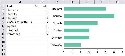
In the comments of Choice of Category Axis Order a reader asked how to use only part of a range as the source data for a chart. Her data and chart initially looked like this:

The line “Total Other Items” is a sum of the items below it in the list, and the chart does not show this subtotal. The series formula looks like:
=SERIES(Sheet1!$B$1,(Sheet1!$A$2:$A$4,Sheet1!$A$6:$A$8),
                    (Sheet1!$B$2:$B$4,Sheet1!$B$6:$B$8),1)
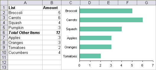
Notice both the X and Y arguments each consist of two ranges, separated by commas, and surrounded by parentheses. The reader inserted some items, both above and below the subtotal line:

The chart does not show the updated data. The series formula looks like:
=SERIES(Sheet1!$B$1,(Sheet1!$A$2:$A$4,Sheet1!$A$7:$A$9),
                    (Sheet1!$B$2:$B$4,Sheet1!$B$7:$B$9),1)
The reader wanted some way to show all of the individual items, and not the subtotal, dynamically or programmatically, to avoid the tedium of updating the chart manually whenever the range was changed. I suggested two ranges, one without the subtotal for charting, and one with the subtotal for the boss. My suggestion was rejected.
I dusted off an old VBA routine which I had originally written to keep zero and blank values out of a chart, and modified it to keep the subtotal line out. The routine redefined some names in the worksheet, and the names were used in the chart. The thing to do is run the routine once, then adjust the chart series formula to this:
=SERIES(Sheet1!$B$1,Book1!myARange,Book1!myMRange,1)
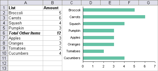
Now whenever thee VBA code is run, it redefines myARange and myBRange. Since the chart series is defined by these, running the code indirectly changes the chart as well. Here is a chart of the table above, updated with the changed names:

Assuming the data is in columns A and B, with headers in row 1 and actual data starting in row 2, and nothing clutters rows A and B beneath the data. This is the macro which, when run whenever the table is changed, will update the chart.
Sub FilterChartSourceDataRange()
  Dim myCell As Range
  Dim myARange As Range, myBRange As Range
  Dim nRow As Long, iRow As Long
  Dim sAvoid As String

  sAvoid = "Total Other Items"

  ' Find last row
  nRow = ActiveSheet.Cells(65536, "A").End(xlUp).Row

  For iRow = 2 To nRow
    Set myCell = ActiveSheet.Cells(iRow, "A")
    If myCell.Value <> sAvoid And Not IsEmpty(myCell) Then
      ' cell is okay, so add to charting ranges
      If myARange Is Nothing Then
        Set myARange = myCell
        Set myBRange = myCell.Offset(0, 1)
      Else
        Set myARange = Union(myARange, myCell)
        Set myBRange = Union(myBRange, myCell.Offset(0, 1))
      End If
    End If
  Next

  ' redefine ranges in worksheet
  ActiveWorkbook.Names.Add Name:="myARange", _
      RefersTo:="='" & ActiveSheet.Name & "'!" & myARange.Address
  ActiveWorkbook.Names.Add Name:="myBRange", _
      RefersTo:="='" & ActiveSheet.Name & "'!" & myBRange.Address

  ' clean up
  Set myCell = Nothing
  Set myARange = Nothing
  Set myBRange = Nothing
End Sub


Colin Banfield says
Hi Jon,
I created a formula based version of this example. It works perfectly in Excel 2003 but not in Excel 2007.
On one machine where I have Excel 2007 exclusively, the category labels don’t show up at all in the chart when I have a discontinuous category range name in the series formula (however, with a static discontinuous range reference, the labels show up fine). If I add another item at the bottom of the list, the value shows up in the chart (sans label).
On another machine, I have both Excel 2003 and Excel 2007 installed. I opened the file I created in the Excel 2007 only machine, and the category labels appear in the chart. However, any new item entered in the list isn’t added to the chart. Sigh!
Jon Peltier says
Excel 2007 doesn’t always deal cleanly with category labels. I haven’t noticed this with dynamic ranges so much as in regular ranges with a lot of data. It’s like I can’t convince Excel to show the labels the way I want. I have no specific example in mind, but I recall agonizing over this, and I’ve answered questions in forums about this.
It also seems harder to build a dynamic range in Excel 2007 than in previous versions. You have to be careful what names you use for the ranges: if the name starts with the word “chart” you cannot manipulate the series formula. But some of this difficulty is using the new dialogs.
Colin Banfield says
Hopefully, this problem is on the list of fixes for SP2. Your particular example is unusual because normally it’s the “Other Items” that is charted (and not the individual items that make up the “Other Items” group).
Anyway, here is a list of the formula names I created:
‘This is the total list range (less header row)
ListRange=OFFSET(Sheet1!$A$1,1,0,COUNTA(Sheet1!$A:$A)-1,2)
‘This is the position of the Total row in ListRange
TotalPos=MATCH(“Total Other Items”,OFFSET(ListRange,0,0,,1),0)
‘This is first category range (before TotalPos)
CatRange1=OFFSET(ListRange,0,0,TotalPos-1,1)
‘This is the second category range (after TotalPos)
CatRange2=OFFSET(ListRange,TotalPos,0,ROWS(ListRange)-ROWS(CatRange1)-1,1)
‘This is the union of CatRange1 & CatRange2
CatRange=CatRange1,CatRange2
‘This is first value range (before TotalPos)
ValRange1=OFFSET(ListRange,0,1,TotalPos-1,1)
‘This is the second value range (after TotalPos)
ValRange2=OFFSET(ListRange,TotalPos,1,ROWS(ListRange)-ROWS(CatRange1)-1,1)
‘This is the union of ValRange1 & ValRange2
ValRange=ValRange1,ValRange2
‘This is the series formula
=SERIES(,Sheet1!CatRange,Sheet1!ValRange,1)
‘This is formula used in the Total row (column 2)
=SUM(ValRange2)
Jon Peltier says
Colin –
Thanks. I was too busy/lazy to work out the defined names, but your approach looks good.
Incidentally, the person who asked me about this figured out the problem using defined names while I was writing this post.
Gustavo says
Dear Jon,
i have a big dude about a code in vba that you create, you wrote that you can filter a listbox with 6 columns and 6 textboxes please i was reading this for long time and i cant imagine how you can do that please if you can share the code i will really appreatiate it
thanks in advance
you write this post about this what i was taking
http://www.dicks-blog.com/archives/2005/02/16/limit-a-listbox/
Jon Peltier says
Gustavo –
Wow, that was four years ago. I don’t remember writing that, nor do I remember which project I was even working on at the time.
You could adjust the code in the Daily Dose article so it compares a particular column of the listbox to the particular textbox. You would define sCrit something like this:
sCrit = "*" & UCase(Me.controls("tbxFind" & j).Text) & "*"then you test the particular item:
Gustavo says
Something like this i tried but it dont work…. any idea???
Private Sub TextBox1_Change()
Dim i As Long
Dim sCrit As String
‘UCase is used to make filter case-insensitive
sCrit = “*” & UCase(Me.Controls(“TextBox1” & j).Text) & “*”
With Me.ListBox1
filfin = Range(“A65536”).End(xlUp).Row
.List = Range(“A2:C” & filfin).Value
For i = .ListCount – 1 To 0 Step -1
If Not UCase(.List(i), j) Like sCrit Then
.RemoveItem i
End If
Next i
End With
End Sub
Jon Peltier says
You got confused with the textbox labeling and the index j and so forth, but here is a more detailed approach.
In each TextBox change event procedures you should call a separate sorting routine, and pass information about the textbox control to the routine.
Private Sub FilterList(iCtrl As Long, sText As String)
    Dim iRow As Long
    Dim sCrit As String

    'Add asterisks around text for all matches
    'UCase is used to make filter case-insensitive
    sCrit = "*" & UCase(sText) & "*"

    With Me.lbxCustomers
        'Start with a fresh list
        .List = vaCustNames
        'Loop through the list backward - always a good
        'idea when you're deleting stuff
        For iRow = .ListCount - 1 To 0 Step -1
            'Remove the line if it doesn't match
            'UCase used again here
            If Not UCase(.List(iRow, iCtrl)) Like sCrit Then
                .RemoveItem iRow
            End If
        Next iRow
    End With
End Sub
Here is what the event procedure would look like this:
Private Sub TextBox1_Change()
    FilterList 1, Me.TextBox1.Text
End Sub
Your textboxes should be labeled starting with 0 (not 1) so that the textbox numbering matches the column numbering in the listbox, which is 0-based.
Kapil bhardwaj says
hello sir,
I have seen your code for making a chart for filter data..
Now I want to use a scroll bar in this logic itself. can you guide me how to do that.
Jon Peltier says
Kapil –
That’s a broad topic which I’ve covered in many posts and web pages. I recommend searching the site for “scrollbar” or “scroll bar”.