Error Bars

I’ve written about Excel chart error bars in Error Bars in Excel Charts for Classic Excel and in Error Bars in Excel 2007 Charts for New Excel. Both articles contained instructions for adding custom error bar values for individual points, but judging from the emails I receive, a separate article on custom error bars is needed. You cannot add custom error bar values to a single point in a chart. However, you can individual custom error bar values to all points in a plotted series. You need to put all of the individual error bar values into a range of the worksheet. I usually put these values in the same table as the actual X and Y values

Manually Defining Custom Error Bars

Sample Data and Charts

Suppose we have the following data: X and Y values, plus extra columns with positive and negative error bar values for both X and Y directions. The data is set up so that, for example, cells C2 and D2 have the values for the positive and negative horizontal (X) error bars for the point defined by X and Y values in A2 and B2. Cells E2 and F2 have the values for the positive and negative vertical (Y) error bars for this point. The series is plotted using all the data at once, with X in A2:A6 and Y in B2:6. The error bars are also drawn using all the error bar data at once: C2:C6 and D2:D6 for horizontal and E2:E6 and F2:F6 for vertical.

The chart itself is easy: create an XY chart using the data in columns A and B.

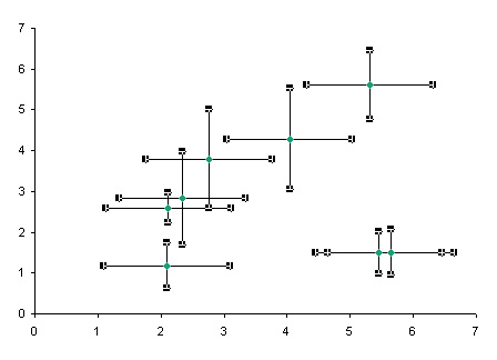
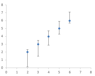
The protocols for adding custom error bars differ between Classic Excel and new Excel. After following the appropriate protocol below, the chart will have custom error bars on each data point, based on the additional columns of data. This chart shows just the Y error bars, to show clearly that each point has custom values different from other points:

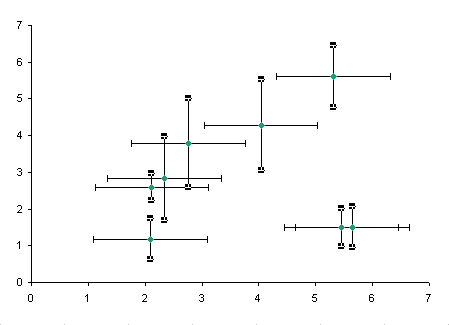
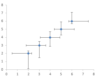
This chart shows the X and Y error bars:

Important Note

A single custom error bar value cannot be added to a single data point, and custom error bar values cannot be added to a series of data points one point at a time. If you select a single value for your custom error bars, this single value will be applied to all points in the series. A whole set of custom error bar values can be added to an entire series in one operation. Put your custom values into a range parallel to your X and Y values as I’ve done with this sample data, then use the manual technique or the utility to add all the values to the chart series in one step.

New Excel (2007 and later)

It is harder to apply error bars in Excel 2007 than in earlier versions. There is no convenient tab on the Format Series dialog. The Error Bar tab(s) as well as the tabs for Data Label, Up/Down Bars, High/Low Lines, and other features have been removed to make them more discoverable, at least that’s what we were told. To discover these features in Excel 2007, select the chart and navigate to the Chart Tools > Layout contextual tab. Click on the Error Bars button, and scratch your head while you try to decipher the options. 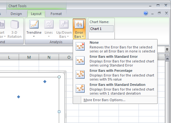Finally, select the More Error Bars Options at the bottom of the list. X (if it’s an XY chart) and Y error bars with initial constant values of 1 are added to the chart series, with the Y error bars selected, and the Format Error Bars dialog is displayed with the Vertical Error Bars tab showing. (If the chart has more than one series, and you had not specifically selected one series, there is an intermediate dialog asking which series to work with.) 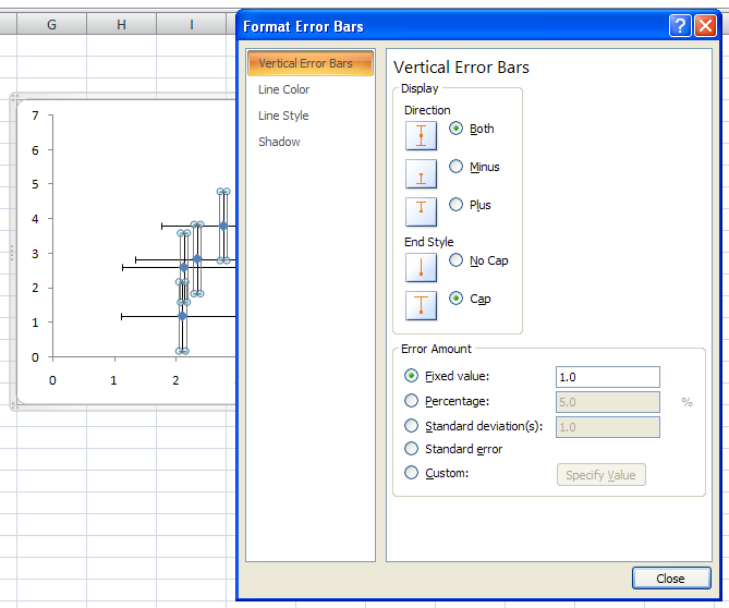This dialog doesn’t look too unfamiliar. But there is no obvious way to switch to the horizontal error bars. We are used to having two tabs, one for the vertical error bars, and also one for the horizontal error bars. Remember that Microsoft made these chart formatting dialogs non-modal, so you can click on objects behind the dialogs. Click on the horizontal error bars to change the dialog. 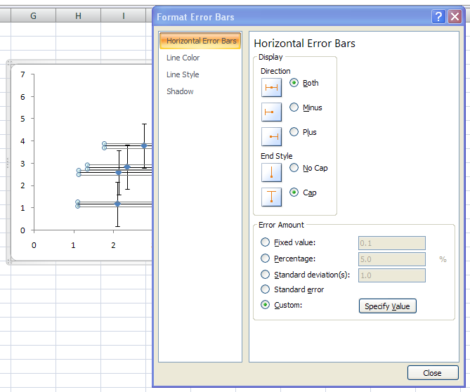To assign custom values to the error bars, select the horizontal or vertical error bars, and on the Horizontal or Vertical Error Bars tab of the Format Error Bars dialog. Move the dialog so it does not cover the range containing your custom values, then click on the Custom option button, and click on Specify Value. A small child dialog appears with entry boxes for selection of the custom error bar values. (It was easier in 2003, where data entry took place directly on the main dialog, but we’re not talking about productivity today.) 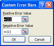By default, each field contains a one element array with the element value equal to one. You can enter another constant value, and you don’t need to type the equals sign or curly brackets; Excel will insert them. More likely you want to select a range. Make sure you delete the entire contents of the entry box before selecting a range, or at least select it all, or Excel will think you meant to enter something like the following, which will lead to an error message. The edit box is so narrow, that you cannot see the entire expression at once, and it will be difficult to find this error.

={1}+Sheet1!$D$2:$D$6

If you want the value to be zero, enter zero. Don’t completely clear an entry box, because Excel will think you simply forgot and it will retain the previous value.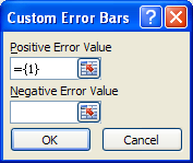

Classic Excel (2003 and earlier)

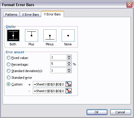
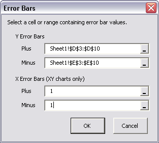
It’s easy to add error bars in Excel 97 through 2003. Bring up the Format Series dialog, by double clicking on the series, by right clicking on the series and choosing Selected Object, by selecting the series and choosing Selected Data Series from the Format menu, or by selecting the series and clicking the shortcut, Ctrl+1 (numeral one). The dialog has a tab for Y Error Bars, and if it’s an XY data series, there is also a tab for X error bars. 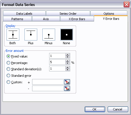To define custom error bars, click in the + or – data entry box (no need to select the Custom option button, Classic Excel does this automatically), then select the range containing the custom error bar values using your mouse. If you need only one value for all of the points, you can select a single cell, or even type the value you want. This seems redundant, given the Fixed Value option, but this way you can use different positive and negative fixed values or a custom range for one direction and a constant for the other. This is what the dialog looks like with ranges used to define the custom error bar values. 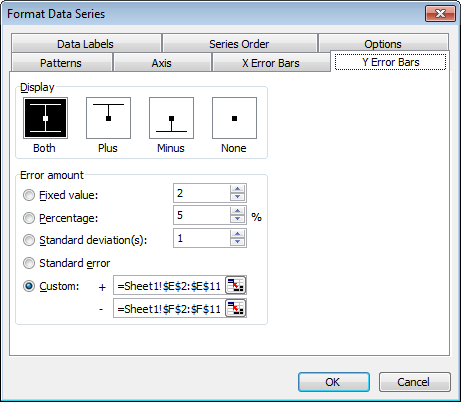If you want to leave an error bar off the chart, you can leave the data entry box blank.

Notes

The error bars overwhelm the data. To restore the importance of the data itself, use a lighter color for the error bars. Lighten up the axes while you’re at it. 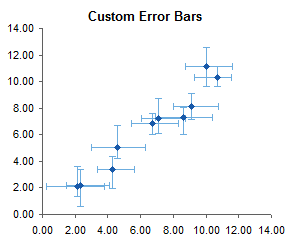If any custom values are negative, the corresponding error bar will be drawn in the opposite direction: a positive error bar with a negative value will be drawn in the negative direction.

Programmatically Defining Custom Error Bars

The command to add error bars using Excel is:

{Series}.ErrorBar Direction:={xlX or xlY}, Include:=xlBoth, Type:=xlCustom, _
    Amount:={positive values}, MinusValues:={negative values}

Values can be a single numerical value, for example, 1, an comma-separated array of numerical values in curly braces, such as {1,2,3,4}, or a range address in R1C1 notation. For values in Sheet1!$G$2:$G$10, enter the address as Sheet1!R2C7:R10C7. Combine both plus and minus in the same command. In Excel 2007, if you don’t want to show a particular error bar, you must enter a value of zero in this command. In 2003, you can enter a null string “”. In Excel 2003, the range address must begin with an equals sign, =Sheet1!R2C7:R10C7; Excel 2007 accepts the address with or without the equals sign. Single values or arrays may be entered with or without the equals sign in either version of Excel.

Error Bar Utility

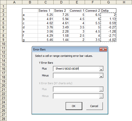
To make it easier to use error bars in Excel 2007 (and in Classic Excel), I’ve built a small utility, which you can download and use for free. It’s found in ErrorBars.zip. This zip file contains two versions, ErrorBars.xls for Excel 97 through 2003, and ErrorBars.xlam for Excel 2007. Install this utility by following the instructions in Installing an Excel Add-In or in Installing an Add-In in Excel 2007. In Classic Excel, the utility places a new item, Add Error Bars, at the bottom of the chart series context menu. All you have to do is right click on the series and select Add Error Bars. Despite all the assurances from Microsoft that context menus work the same in Excel 2007 as in earlier versions, you cannot add an item to an Excel 2007 chart-related context menu. What I’ve done instead is to add an Error Bars item to the end of each of the three Chart Tools contextual ribbon tabs. I know the new philosophy of Office is to place a command in only one place in the whole user interface. I prefer the old style philosophy, however, which is to place the command in every place it may be relevant. I never know where I may be when I want to use a command, and some people remember different hiding places than I do. 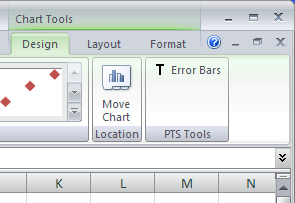Whether in Excel 2007 or in earlier versions, click on the added command, and the utility behaves the same. Up pops a simple dialog with four data entry boxes, for plus and minus Y error bars, and for plus and minus X error bars. 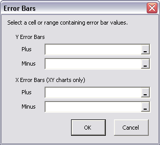If the chart type is not XY, the X error bar entry boxes are disabled. 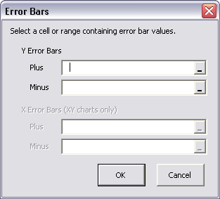You can select a range or enter a constant into the entry boxes. Leave a box blank to omit the corresponding error bars. I hope that this tutorial and the associated utility will make your life easier when working with error bars in Excel 2007.