Apply an AutoFilter to an Excel Pivot Table
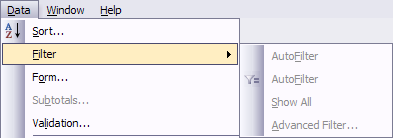
Excel Pivot Tables are a very powerful feature, and the AutoFilter is also very useful. The row fields of the Pivot Table can be manipulated like an AutoFilter, but the data fields cannot be sorted or filtered. And if you try to apply an AutoFilter to a pivot table, you find the menu command disabled.

But I learned a trick this week at the Excel Dashboard and Visualization Bootcamp. If you select a cell which borders on the pivot table, but is not part of the pivot table,…

…the AutoFilter menu items are now enabled.

Select AutoFilter, and the Pivot Table has been AutoFilter enabled.

These conferences are great.
AutoFilter by Selection
Access has a feature that lets you quickly apply a filter based on the selected item. Wouldn’t it be great to have this in Excel?
Well, this feature exists, and it’s built in. But it’s not present on the default menus or ribbons. You have to dig it out and install it yourself.
Excel 2003 and earlier
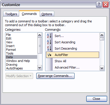
On Excel’s Tools menu, select Customize, click on the Commands tab, select the Data item in the Caegories list, click on the AutoFilter item, and drag it to a convenient place on a toolbar or menu.

I’ve put this just under the “regular” AutoFilter item on my Data menu/Filter submenu.

Excel 2007
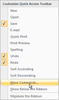
Click on the down arrow to the right of the Quick Access Toolbar, and select More Commands from the popup menu.

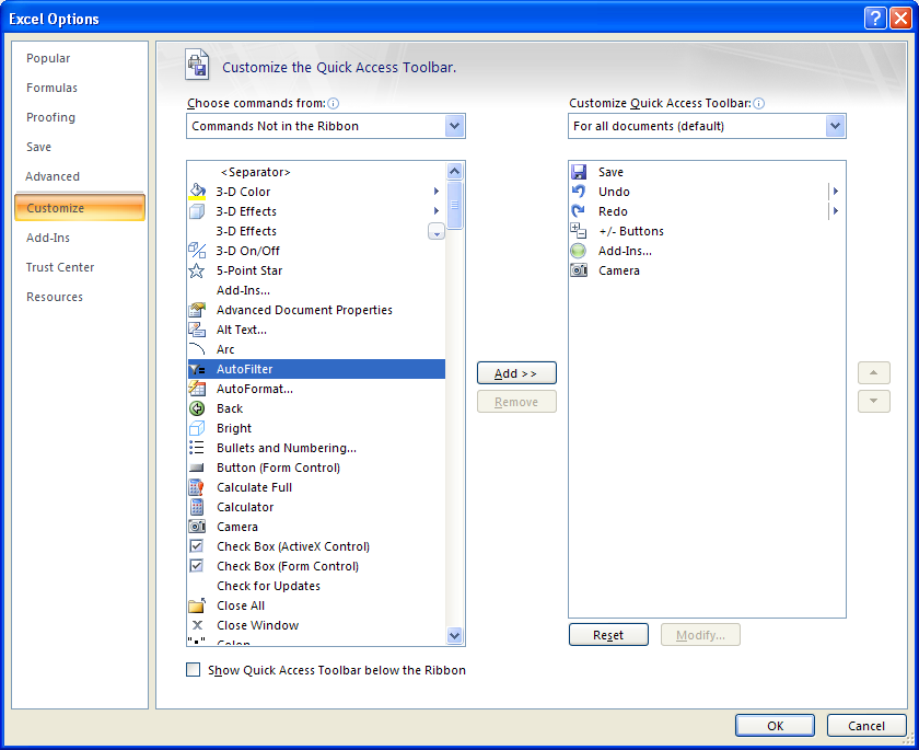
In the oversized dialog that appears, select Commands not in the Ribbon from the right hand dropdown, select AutoFilter, click Add, and press OK.

The AutoFilter icon appears on the QAT.

What the “New” AutoFilter does
This Autofilter command shares a name with the “other” AutoFilter command, but it has a unique icon, and its functionality is enhanced. The command creates an AutoFilter using the range that includes the active cell, then it filters this range based on the active cell.


