Stack Columns In Order Of Size With VBA

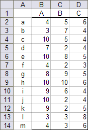
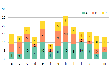
In Stack Columns In Order Of Size I showed a worksheet formula approach to sort columns in each stack in a stacked chart by size, not by series. When you create a stacked column chart the usual way, the columns are stacked in the same series order, as shown below.

– – –

This technique required seven columns of intricate calculations to portray the three series, the columns of formulas increase faster than the number of visible series in the chart, and the formulas become longer as series are added. Too much tedium, too many chances to mess it up.

Programmatic Approach

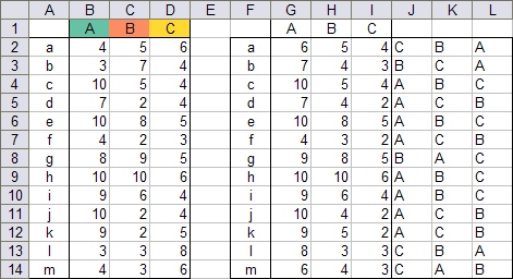
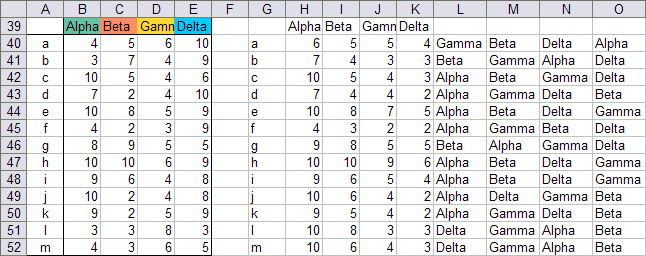
So I build a simple VBA routine. A1:D14 is the input data (the data need not start in A1). The first row contains series names and the cells are filled with the color to format the data points in the chart. The first column holds the category labels, and the data to be sorted and plotted is in B2:D14.

F1:L14 is the output data. The category labels and series names are copied over from the input range. (The bottom series in the chart is labeled with the first series name, regardless of which column of the original data provides the points for this series.) Each row of data values has been sorted left to right in decreasing order in G2:I14, and the series name corresponding to a particular data value is placed in the same cell within the range J1:L14.

Here is the chart created by the program.

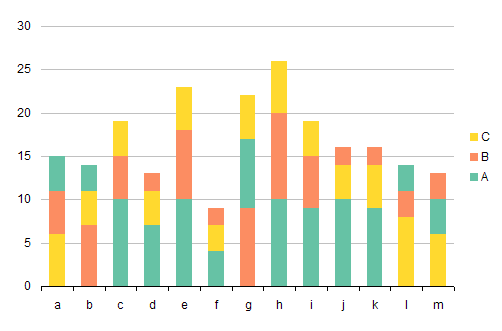
This procedure works just as well if there are four or more initially columns of data, unlike the manual worksheet formula version, which is already getting bogged down at three columns.

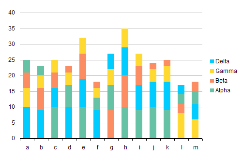
Frankly, I’m not sure the charts with sorted columns are easier to read. In fact, when they are sorted it’s easier to keep track of which value goes with which series. With the blocks in different order for each stack, you have to keep referring to the legend. This negates any possible benefit of the blocks being in numerical order.

The VBA code is shown below. The procedure ProcessInputRange does all the work in the range passed to it. The procedure ProcessInputRangeSelection is run from Excel: it finds the selected range and passes it to ProcessInputRange. I separate my code into pieces like this to make it easier to reuse the pieces. For example, I could call ProcessInputRange from a different routine, perhaps cycling through all the sheets in a workbook and processing all of the data.

Sub ProcessInputRangeSelection()
  If TypeName(Selection) = "Range" Then
    ProcessInputRange Selection
  End If
  ActiveSheet.Cells(ActiveWindow.ScrollRow, ActiveWindow.ScrollColumn).Select
End Sub

Sub ProcessInputRange(rInput As Range)
  ' range- and array-related
  Dim vaInput As Variant
  Dim vaYValues As Variant
  Dim vaXValues As Variant
  Dim vaNames As Variant
  Dim vaLabels As Variant
  Dim vYValueTemp As Variant
  Dim vLabelTemp As Variant
  Dim nXValues As Long
  Dim nNames As Long
  Dim iRow As Long
  Dim iCol As Long
  Dim iCol1 As Long
  Dim iCol2 As Long
  Dim rOutput As Range
  ' chart-related
  Dim lLeft As Double
  Dim lTop As Double
  Dim lWidth As Double
  Dim lHeight As Double
  Dim cht As Chart
  Dim iSeries As Long
  Dim iPoint As Long
  Dim vaColor As Variant

  vaInput = rInput.Value2

  nXValues = UBound(vaInput, 1) - 1
  nNames = UBound(vaInput, 2) - 1

  ReDim vaNames(1 To 1, 1 To nNames)
  ReDim vaXValues(1 To nXValues, 1 To 1)
  ReDim vaYValues(1 To nXValues, 1 To nNames)
  ReDim vaLabels(1 To nXValues, 1 To nNames)

  ' populate arrays
  For iRow = 1 To nXValues
    vaXValues(iRow, 1) = vaInput(iRow + 1, 1)
  Next
  For iCol = 1 To nNames
    vaNames(1, iCol) = vaInput(1, iCol + 1)
  Next
  For iRow = 1 To nXValues
    For iCol = 1 To nNames
      vaYValues(iRow, iCol) = vaInput(iRow + 1, iCol + 1)
      vaLabels(iRow, iCol) = vaNames(1, iCol)
    Next
  Next

  ' bubble sort values in each row, sort labels at same time
  For iRow = 1 To nXValues
    For iCol1 = 1 To nNames - 1
      For iCol2 = iCol1 + 1 To nNames
        If vaYValues(iRow, iCol2) > vaYValues(iRow, iCol1) Then
          vYValueTemp = vaYValues(iRow, iCol1)
          vaYValues(iRow, iCol1) = vaYValues(iRow, iCol2)
          vaYValues(iRow, iCol2) = vYValueTemp
          vLabelTemp = vaLabels(iRow, iCol1)
          vaLabels(iRow, iCol1) = vaLabels(iRow, iCol2)
          vaLabels(iRow, iCol2) = vLabelTemp
        End If
      Next
    Next
  Next

  ' put adjusted arrays into worksheet
  Set rOutput = rInput.Resize(1, 1).Offset(, nNames + 2)
  rOutput.Offset(, 1).Resize(, nNames).Value = vaNames
  rOutput.Offset(1).Resize(nXValues).Value = vaXValues
  rOutput.Offset(1, 1).Resize(nXValues, nNames).Value = vaYValues
  rOutput.Offset(1, 1 + nNames).Resize(nXValues, nNames).Value = vaLabels

  ' get colors
  With rInput.Offset(, 1).Resize(1, nNames)
    ReDim vaColor(1 To 1, 1 To nNames)
    For iCol = 1 To nNames
      vaColor(1, iCol) = .Cells(1, iCol).Interior.ColorIndex
    Next
  End With

  ' process chart
  lWidth = ActiveWindow.UsableWidth / 2
  lHeight = ActiveWindow.UsableHeight / 2
  lLeft = ActiveSheet.Columns(ActiveWindow.ScrollColumn).Left + lWidth / 2
  lTop = ActiveSheet.Rows(ActiveWindow.ScrollRow).Top + lHeight / 2

  Set cht = ActiveSheet.ChartObjects.Add(lLeft, lTop, lWidth, lHeight).Chart

  With cht
    .SetSourceData Source:=rOutput.Resize(nXValues + 1, nNames + 1), PlotBy:=xlColumns
    .ChartType = xlColumnStacked

    .ChartGroups(1).GapWidth = 100
    With .PlotArea
      .Border.LineStyle = xlNone
      .Interior.ColorIndex = xlNone
    End With
    With .Axes(xlValue)
      .Border.LineStyle = xlNone
      With .MajorGridlines.Border
        .ColorIndex = 48
        .Weight = xlThin
      End With
    End With
    .Legend.Border.LineStyle = xlNone
    With .ChartArea
      .Border.LineStyle = xlNone
      .AutoScaleFont = False
      .Font.Size = 9
    End With

    ' format points
    For iSeries = 1 To nNames
      With .SeriesCollection(iSeries)
        .Border.LineStyle = xlNone
        .Interior.ColorIndex = vaColor(1, iSeries)
        For iPoint = 1 To nXValues
          For iCol = 1 To nNames
            If vaLabels(iPoint, iSeries) = vaNames(1, iCol) Then
              .Points(iPoint).Interior.ColorIndex = vaColor(1, iCol)
              Exit For
            End If
          Next
        Next
      End With
    Next

  End With

End Sub

To use the program, select your input data range, press Alt+F8 to bring up the Macro dialog, select ProcessInputRangeSelection, and press Run.