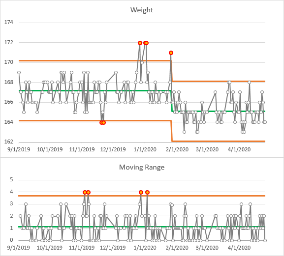
Use Power Query to Manipulate Your Data

Last week, I wrote about Watching my Weight with SPC (Statistical Process Control).

I followed that post with with Dynamic Arrays, XLOOKUP, LET where I showed off some new Excel features that made it easy to manipulate my data so I could plot the data in a box plot.

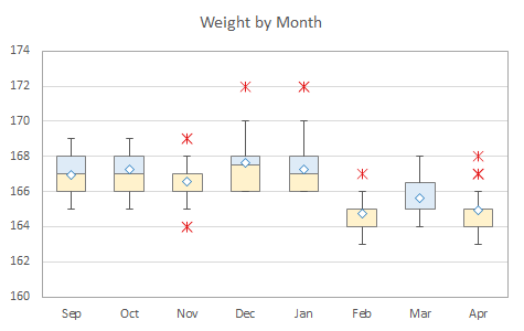
Following the theme of Excel is Evolving, Are You? I’ve decided to show how to use Power Query to perform these same manipulations.

The Data

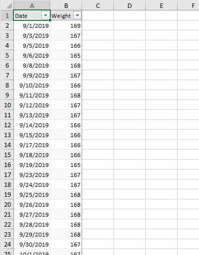
My data data is in a two-column Table of dates and corresponding weights; I’ve named the Table DataDateWeight. In my last article, I used a combination of Dynamic Arrays, XLOOKUP, and the new LET function to build a table in the worksheet, starting in cell D2, which has month as column headers and day numbers in the first column of each row. This will produce a grid of weights with a few missing values. I can feed this directly into Peltier Tech Charts for Excel, the VBA add-in I use to make box plots.

Get and Transform aka Power Query

Power Query is a powerful set of tools that let you import data from a variety of places and then manipulate that data to make it useful. In their infinite wisdom, Microsoft has incorporated Power Query into Excel (as well as Power BI); in their infinite ability to confuse, they have renamed the Excel version Get and Transform. They’re really synonyms, since what Power Query does is Get and Transform data.

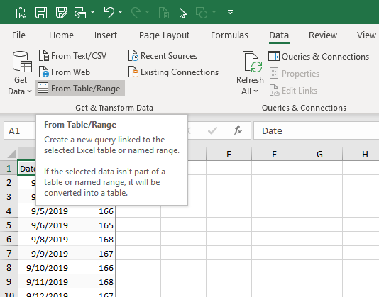
Power Query makes up the left portion of Excel’s Data tab. If you click the Get Data down arrow, you expose a cascading menu of data sources, including From Table/Range, which we’ll use to manipulate our data which is already in Excel.

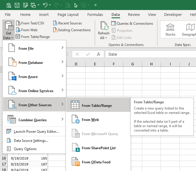
You can also just click the From Table/Range button on the ribbon.

The Power Query Editor

This opens up the marvelous and at first scary Power Query Editor. We see the contents of our Table in the editor window. Over in the task pane on the right, I have renamed the Query to DateWeight (the default query name is the name of the source Table).

The Applied Steps section in the task pane shows the contents of this query that I’m writing. So far we see Source and Changed Type. When we started, Power Query used the Table as its source, then applied its best guess at what data type was present in each column. Looks good, as we can see from the Date and 123 (whole number) icons in the header row.

The formula bar shows the current operation, in a specialized language called M Code. For the most part, you don’t need to be too concerned with these formulas, at least not until you’ve become familiar with Power Query.

At any time, I can go back and click on a previous step, and Power Query will update the window to show the state of the data at that step, with that step’s M Code in the formula bar. I can also go back and insert or remove a step, taking care not to break my whole query in the process.

I need a column with the day of the month, and I need to transform the Date column to the month abbreviations. Then I need to pivot the month abbreviations so I end up with one column for each month.

Adding a Column

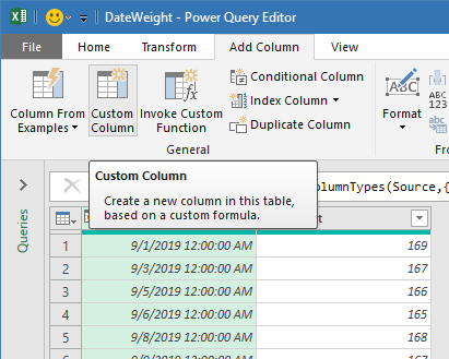
Let’s start with the day of the month. Click Custom Column on the Add Column tab of the ribbon.

This pops up a Custom Column formula editor.

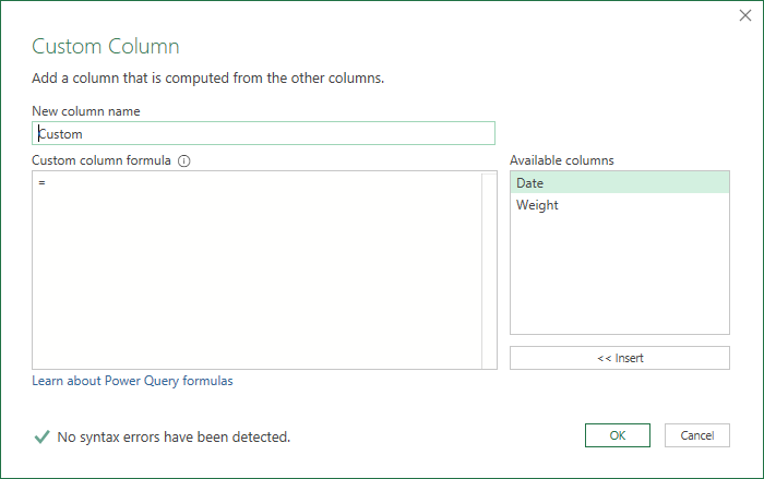
Power Query has an amazing IntelliSense system, as you’ll see.

First I changed the new column name to Day. Then I typed day after the equals sign. Power Query shows a list of possible commands matching the word day, and I scrolled down until I found Date.Day.

Entering a Formula in Custom Column Dialog

I clicked on Date.Day, which Power Query inserted into the formula, and it popped up a description of what I needed to use in this formula. There’s also a hint at the bottom of the window next to the yield icon. What I need is the Date column, which appears in the list on the right.

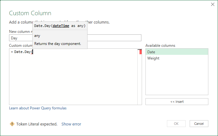
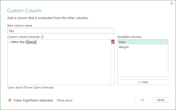
Editing a Formula in Custom Column Dialog

Double clicking on the Date column in the list enters it in the formula. Power Query updates the yield icon warning to say I need a closing parenthesis. Actually it says Token RightParen expected, but pretty soon you’ll learn what these messages mean.

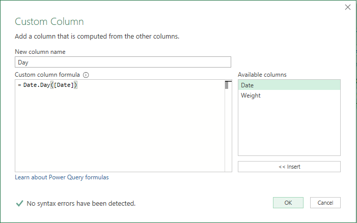
Type the closing parenthesis, and the icon changes to a green checkmark, and the message becomes surprisingly comprehensible, No syntax errors have been detected.

Click OK and the column is added. Congratulations, you’ve just written your first statement in M Code. Note the new Added Column entry under Applied Steps.

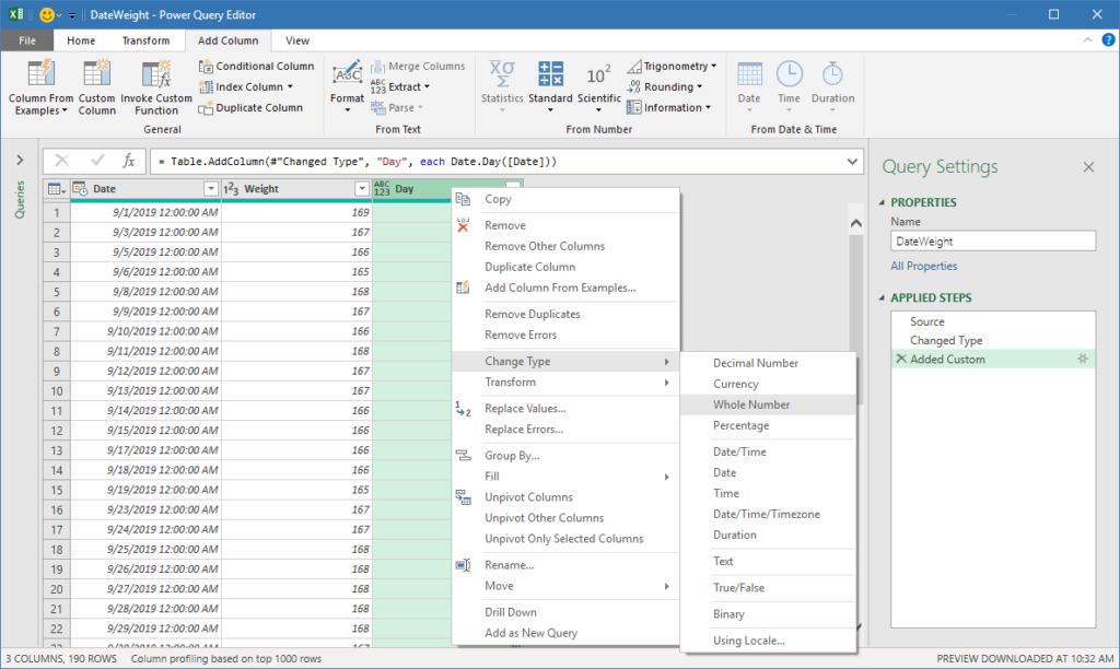
The abc icon in the new column header indicates that the Day column is formatted as text. Right click the column header, choose Change Type > Whole Number.

Custom Column Has Been Added — *click to enlarge*

The icon changes to the 123 whole number icon. That’s another M Code statement, by the way. You didn’t even know you were writing it, but Power Query records every step you take, so you can repeat the query, or edit it as your model evolves.

Convert Date to Month Abbreviation

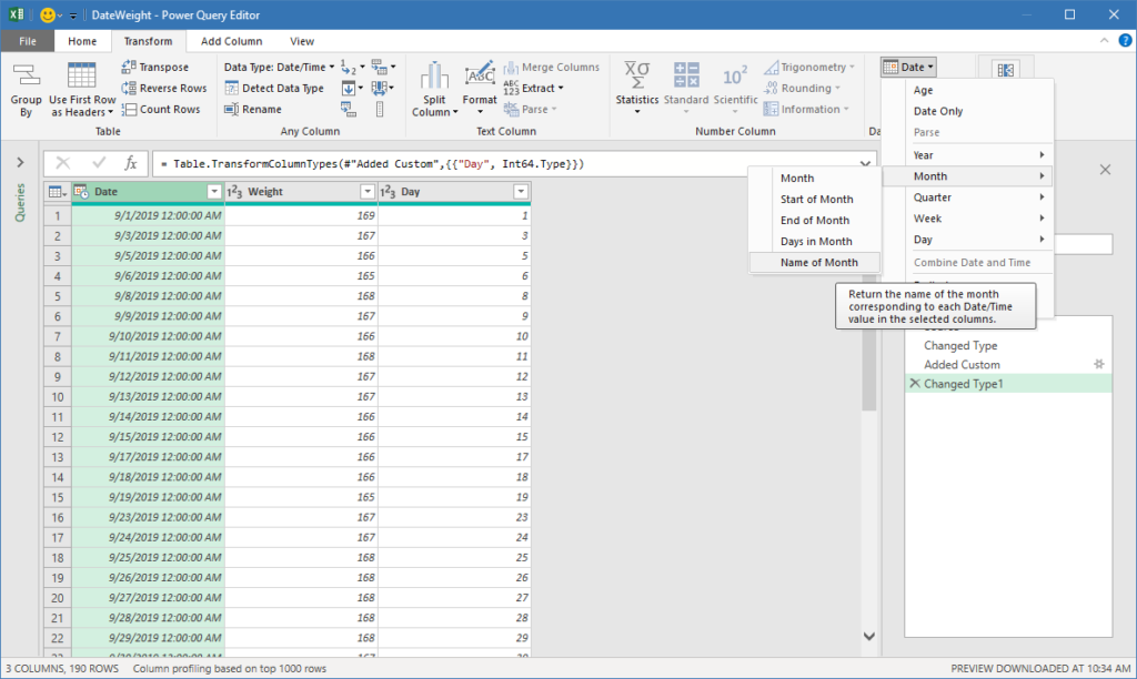
We can transform our Date column in place. On the Transform tab, click on Date, then choose Month > Name of Month.

Our dates have been converted into month names, and the data type icon has changed from a miniature calendar to the abc text icon. Nice, now let’s abbreviate it. On the Transform tab, click Extract > First Characters.

Month Name to Abbreviation — *click to enlarge*

In the Extract First Characters dialog, enter 3, then click OK.

The month names are now abbreviated.

Pivot by Month

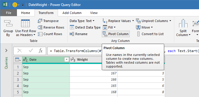
With the Date column still selected, click on Pivot Column on the Transform tab.

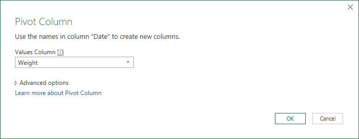
The Pivot Column dialog asks which column to use for values. If we made a Pivot Table in regular Excel, Month would be in the Columns area, Day in the Rows area, and Weight in the Value area. So select Weight and click OK.

Pivot Date Column Using Weight for Values

Power Query pivots our months into column headers, and it looks like we’re done with our query. The column data types are all 123 whole numbers, and everything looks great.

The Advanced Query Editor

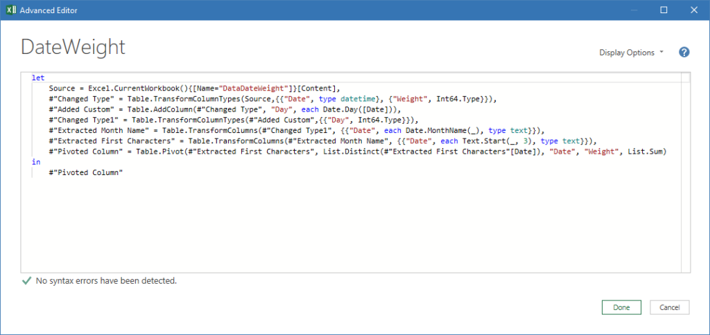
Click on the Advanced Editor button on the Home tab.

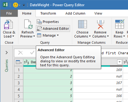
The Advanced Editor shows our entire query in M Code. If we wanted to and if we were smart enough, we could edit the code here.

Advanced Query Editor — *click to enlarge*

Put the Data Back into Excel

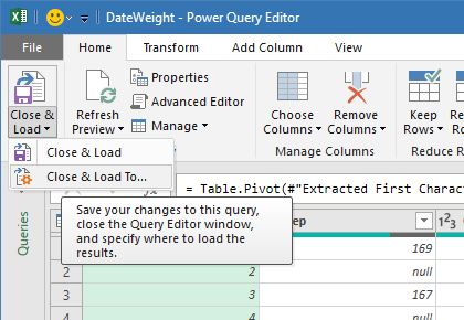
It’s time to put the data back into Excel, so we can do something useful with it. The first button on the Home tab is Close & Load. We’re going to load the query into a Table on our worksheet. Out of the box, Power Query’s default is to load into a Table, but you can change your default. My default is to load the data into the workbook’s Data Model (like an advanced pivot cache) without a Table, so I’ll click Close & Load To…

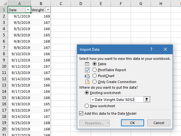
In the Import Data dialog, I’ve clicked Table and selected the cell where I want my Table to go.

Click OK and wait a moment for Excel to refresh the query, and the Table appears. Power Query Tables use green formatting instead of the default Excel blue.

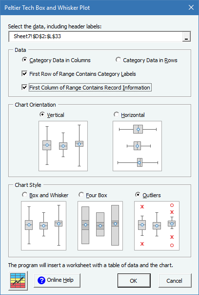
Now all I have to do is select the Table and insert my box plot.

Peltier Tech Charts for Excel Box Plot Dialog

The query does not immediately update when the data changes, so it’s not dynamic the way my formula-based approach from the previous tutorial. However, I can refresh the query using the Refresh button on the Ribbon, or by right-clicking on the Table and choosing Refresh from the pop up menu.

Queries & Connections

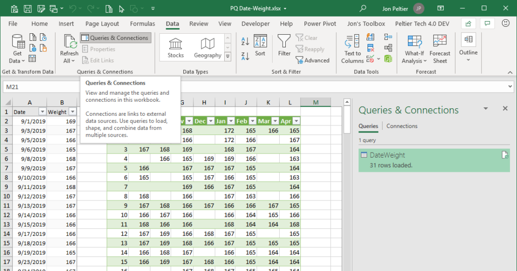
I can get to any queries in my workbook by clicking Queries & Connections on the Data tab, which pops up a task pane.

When I mouse over the query in the task pane, a preview of the query pops up, showing a portion of the query results and some information about the query. I can also edit or delete the query here, and take other actions. If a query is deleted, the table remains in the worksheet, but it is no longer linked to the query or its underlying data.