By definition an interactive dashboard contains methods for users to control which information is displayed. This can be accomplished in many ways. In Interactive Charting by Combo Box or Checkbox I wrote about using checkboxes and worksheet formulas to do this, and I elaborated on the technique in Interactive Charts with Checkboxes and Formulas.
There are a couple of shortcomings with the checkboxes-plus-formulas approach. If a series is not displayed, there is still a space for its bars in a column chart. Also, the legend key (marker in the legend) for the series is still present even if the label is hidden.
By using VBA and checkboxes together, these shortcomings can be avoided. This technique makes use of Excel’s default behavior, which does not show data in a chart if the data range is hidden. This behavior can be changed on a chart by chart basis, so that changing it for one chart does not change it for other charts.
Checkboxes and VBA
Start with a line or column chart that includes all of the series you will allow the user to select from (A, B, and C in this example). Add a checkbox from the Forms toolbar for each series.
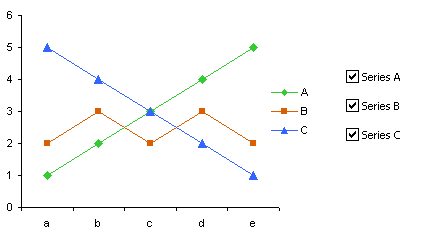
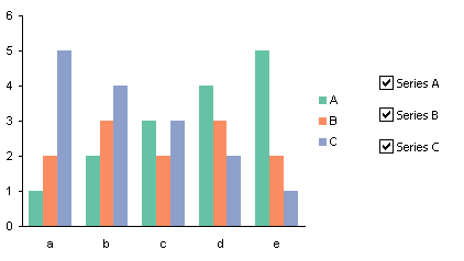
The data is very simple, as shown below. The source data for the chart is in range J3:M8, and K1:M1 are the cells that the checkboxes are linked to. The range K1:M1 is named “TrueFalseRange” (select the range, click in the Name Box and type TrueFalseRange, and press ENTER).
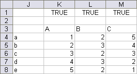
In addition to the checkboxes being linked to cells in the TrueFalseRange, each is also assigned to a macro named ClickSeriesTextbox. The macro is very simple:
Sub ClickSeriesCheckbox()
    Dim rCell As Range
    For Each rCell In ActiveSheet.Range("TrueFalseRange").Cells
        rCell.EntireColumn.Hidden = Not rCell.Value
    Next
End Sub
All this macro does is check each cell in TrueFalseRange, if the value is False it hides the whole column, otherwise the column is displayed.
When (for example) the checkbox for Series B is unchecked, column L is hidden (signified by the thicker line between the column headers for columns K and M).
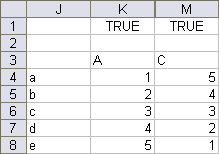
Series B is completely eradicated from the charts, leaving behind no spurious legend key, and no empty slot for Series B’s columns in the column chart.
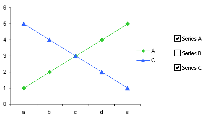
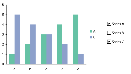
If the user unchecks all of the checkboxes, all of the series value columns are hidden (note the darker line between the headers for columns J and N).
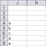
Not only are all series removed from the charts, but so are the axes, titles, legends, and other chart features. The chart is only visible in this screen shot because it has been activated.

CheckboxAndVBA.zip is a zipped workbook that illustrates this technique.


Lawrence says
Hi,
Your Web pages have been VERY helpful. Thank you!
One question on the “Interactive Charts with Checkboxes and VBA” macro. I copied it to my own worksheet and changed it from hide column to hide row. But it only works successfully when I manually run the macro and not automatically when a cell in the true/false range is changed.
What am I doing wrong? I’m not very familiar with VBA, so be gentle.
Thanks again.
Lawrence
Jon Peltier says
Note in the VBA procedure, it references the range “TrueFalseRange”, which contains the cells which are modified by the checkboxes. You would have to make sure to change the alignment of your TrueFalseRange so that a change in this range results in the appropriate row being changed.
Lawrence says
Jon,
I changed the range name and the range in both the worksheet and in the VB editor. But when I change one of the true/false cells nothing happens. The macro will only run (and run correctly) after I click on the run macro button up on my toolbar. How do I get the macro to run the instant one of the true/false cells is changed?
Here’s more detail… My true/false range is D36:D39 and it is named “Chart5TrueFalseSeriesRange”. Then, I copied your macro into a module 1 of my workbook and changed 2 things: the macro name; and rCell.EntireColumn.Hidden to rCell.EntireRow.Hidden.
So, the macro looks like this:
Option Explicit
Sub Chart5HideSeriesCheckbox()
Dim rCell As Range
For Each rCell In ActiveSheet.Range(“Chart5TrueFalseSeriesRange”).Cells
rCell.EntireRow.Hidden = Not rCell.Value
Next
End Sub
If it helps, I can send you the 1-page workbook.
Thanks again!
Lawrence
Lawrence says
Oh, one other detail. My check boxes are ActiveX controls.
Lawrence
Jon Peltier says
Lawrence –
You need to tell the checkbox event code to run your procedure. In design mode, right click on a checkbox and select View Code. This creates an event procedure stub in the code module of the parent worksheet that will fire when the checkbox is clicked. Insert the procedure in this stub (as follows) so the click will run the code.
Private Sub CheckBox1_Click()
Chart5HideSeriesCheckbox
End Sub
Lawrence says
Jon,
I entered the code as instructed and when I click on the checkbox I get “Compile error: Syntax error”.
The original code is located in Module1 and the new code to fire the macro is located in parent worksheet in the VB Editor called Sheet 3 (Data).
Lawrence
Jon Peltier says
Lawrence – What is highlighted in the code module?
Lawrence says
Jon,
When I click on the checkbox1 and I get the error, it opens up the VB Editor and the second line of the macro is highlighted, Chart5HideSeriesCheckbox().
The whole macro in Sheet3(Data) is 3 lines:
Private Sub CheckBox1_Click()
Chart5HideSeriesCheckbox()
End Sub
The macro in Module 1 is unchanged from the comment above.
Lawrence
Jon Peltier says
The error indicates that it can’t find Chart5HideSeriesCheckbox(), or that there is some other kind of syntax error involved. Remove “()” from the line that calls the sub, so all that appears is the name of the sub.
Lawrence says
SUCCESS!
Thank you.
Now that I have the checkboxes working on the Data worksheet, I will need to move them to the worksheet where the chart will be moved to. Will the checkboxes be able to reveal/hide rows on the “Data” worksheet if they are located on the “Dashboard” worksheet? I tried it after I moved the code to the Dashboard tab; the linked cell works on the Data tab, but the row will not hide. Does that have something to do with the part Module1 code that says ActiveSheet? If so, do I simply replace that word with “Dashboard”?
Man, this is so much fun when cool tools like this work so beautifully!
Lawrence
Jon Peltier says
Lawrence –
It will work as long as you can keep track of which button is where, that its event code is on the module behind this sheet, and the code that does the hiding hides the proper ranges on the proper sheet.
Lawrence says
Jon,
Everything is now working perfectly. YAY!!!
My only question is whether the code that I changed slightly makes for “good code”. I simply deleted the text “ActiveSheet.” from before the Range stuff in the 3rd row:
Sub Chart5HideSeriesCheckbox()
Dim rCell As Range
For Each rCell In Range(“Chart5TrueFalseSeriesRange”).Cells
rCell.EntireRow.Hidden = Not rCell.Value
Next
End Sub
Will that change result in problems down the road?
Lawrence
Jon Peltier says
Lawrence – At first glance, it looks okay.
DaleW says
Jon – Thank you for providing the “missing manual” on how to make great Excel charts. This chapter on designing interactive charts — with or without any VBA code — was perfect for my main project today.
Sherman says
Hi Jon, thanks for this!
I am using this code in Excel 2010 and it runs really slow after I check/uncheck boxes while using form control, it takes 10-15 seconds to run when I am only using it to show/hide 20 columns. Is there something I am doing wrong?
Sherman
bs0d says
I happened upon this article while searching for Excel vba info.
In Excel 2013, You can select the chart and set the format.line.visible property to msoFalse. Here is a code sample;