Hinge Techniques for Determining Quartiles

This is the second of a five part series.

Quartiles for Box Plots

This topic is covered in the companion page Quartiles for Box Plots.

Hinge Techniques for Determining Quartiles

Hinges represent an easy definition for quartiles of a data set. Arrange the values in the shape of a “W”, with equal length legs.

The central value of the data set is the value at the peak in the middle of the W, in this case, 5.

The values at the bottoms of the W, 3 and 7, are called Hinges, and they serve as quartiles in this simple definition.

A data set makes a neat W if the number of points N can be defined by

N = 4k + 5

where k is a positive integer. For k=1, N=9, as in the example above. For k=2, N=13. A data set of 13 values is shown below.

Alternative Hinge Definitions

To make it easier to explain and comprehend the discussions that follow, the data sets will be laid out along a number line such as this:

The gray numbers under the number line correspond to locations along the length of the set of values (as a continuous variable), while numbers above the number line correspond to the index of a particular value of the data set. A fractional number above the number line indicates that the resulting value is interpolated between the adjacent values.

Using a W-shaped data layout works for some sizes of data sets, but how can we define hinges for any arbitrarily sized data set? Such a set is shown below; it has 9 values, which we solved above, but we will use it to illustrate the general case.

We can define the Median as the middle value of the data set, as always. We can define the lower hinge as the median of the bottom half of the data, and the upper hings as the median of the top half of the data. Sounds easy, right?

Inclusionary Hinge Definition (“Tukey”)

When John Tukey was laying out his first box plots, he decided that the central data point (the median) of an odd-numberd data set should be included with both lower and upper halves of the data when determining the medians of these halves, that is, when determining the hinges.

As in the “W” layout example above, the median of this 9-value example is 5, while the hinges are at 3 and 7.

Tukey’s name is generally associated with this definition of hinges.

Exclusionary Hinge Definition (“Moore and McCabe” or “M&M”)

Some statisticians didn’t like the idea of the median being counted twice by being part of both the bottom and top halves of the data. Besides, it already has an important role as Median of the data set.

These people thought that the hinges should be defined as the medians of the upper and lower halves of the data set, excluding the median. In the 9-value example, the Median is unchanged at 5, but now the hinges are 2.5 and 7.5.

This exclusionary approach to hinges is often referred to by the names of two of its proposers, Moore and McCabe, or M&M if you like candy.

If the data set has an even number of values, of course, there is no distinction between the inclusionary and exclusionary definitions, as there is no central median value to include or exclude.

Empirical Distribution Function (“CDF”)

For data sets with an even number of observations, the inclusionary (Tukey) hinges and the exclusionary (M&M) hinges are the same. For odd numbers of values, the inclusionary hinges are always closer to the median than the exclusionary hinges.

A third approach is a compromise between the Tukey and Moore-McCabe approaches. Called the Empirical Distribution Function or the Cumulative Distribution Function, or referred to by its initials CDF, it says in the case of an odd number of values in the data set, include the central median if including it will result in odd-numbered halves, and exclude the central median if excluding it will result in odd-numbered halves. This compromise results in actual values from the data set (as opposed to averages of two adjacent values) being used as hinges most of the time.

The CDF technique is the default quartile method used by the statistics package SAS, where it’s called “Empirical Distribution Function with Rounding”.

All Possible Cases of N

We can’t always lay the data out in a “W” shape. Since we’re dealing with splitting a data set into four parts, we only need to consider four cases: when the number of values N is evenly divisible by 4, or when the remainder of this division is 1, 2, or 3. These can be written as

N = 4k
N = 4k + 1
N = 4k + 2
N = 4k + 3

We will look analyze 8 (4k), 9 (4k+1), 10 (4k+2), and 11 (4k+3) values. Nine values here is a repeat of the Tukey and M&M illustration above.

8 (4k) Values

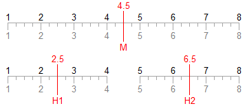
Here is our number line with a set of 8 (4k) observations.

The median is the average of the two values closest to the center, that is, 4.5.

The lower hinge is the average of the two central values in the bottom half of the data, 2.5. The upper hinge is the average of the two central values in the top half of the data, 6.5.

No need to hurt our brains deciding whether to include or exclude the global median from determination of the hinges. The hinges are the same for all three methods for N=4k.

9 (4k+1) Values

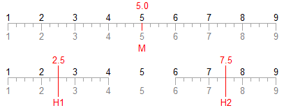
The 9 (4k+1) observation data set leads to two results, depending on whether the central median value is included or excluded from determination of the hinges. In both cases, the median is the central value, or 5.

In the inclusionary (Tukey) approach, the hinges are the midpoints of the data halves, or 3 and 7.

In the exclusionary (M&M) approach, the hinges are the averages of the two central values of each half of the data set, 2.5 and 7.5.

The CDF and Tukey hinges are in agreement for N=4k+1. The M&M values are slightly further from the median.

10 (4k+2) Values

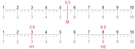
In the 10 (4k+2) observation sample, the median is the average of the two central values, or 5.5.

The lower and upper hinges are the central values of the bottom and top halves of the data set, 3 and 8. No worries about the global median value here.

The three hinge definitions all agree on the hinge values for N=4k+2 values.

11 (4k+3) Values

The 11 (4k+3) observation data set leads to two results, as in the 9 (4k+1) obervation data set. In both cases, the median is the central value, or 6.

In the inclusionary determination, the hinges are the averages of the two central values of each half of the data, 3.5 and 8.5.

In the exclusionary (M&M) approach, the hinges are the central values of the two halves of the data set, 3 and 9.

The CDF and M&M hinges are the same for N=4k+3, with the Tukey hinges lying slightly closer to the median.

Interpolation Methods of Determining Quartiles

This topic is covered in the companion page Quartiles.

Comparison of Values from All Hinge and Quartile Methods

This topic is covered in the companion page Comparison.

Quartiles in the Peltier Tech Chart Utility

This topic is covered in the companion page Quartiles in the Peltier Tech Chart Utility.