Extend Range to Add New Series (VBA)

In some of the analyses I do, I’ll have a range of data and some charts based on this range. As the analysis unfolds, more columns may be added to the data range, and these have to be added to the chart. Until last week, I would add a series by copying the series formula of an existing series, selecting the plot area, pasting the formula into the formula bar, editing the formula, and pressing Enter. Adding series has been the most tedious part of the analysis, and finally I decided to speed it up.

I wrote some code to create a new series based on the range next to the last series in the chart. The code copies the series formula from the last series, then edits the formula to reference the next column for the name and Y value parameters of the formula. Finally a new series is created, and the edited formula is assigned to this series.

Wonderful! One click to add each new series. Well, a few clicks, but it’s still much faster than the old way.

Then I embellished the routine, added some checks (is a chart selected, is the series formula well-formed, are the ranges readily manipulated, etc.), generalized it to series by rows as well as by columns, and ran a few tests. Worked like a charm.

Here’s a sample chart which initially uses the first three data columns as the Y values for its three series. (With the plot area or chart area selected, the source data range for the chart is highlighted.)

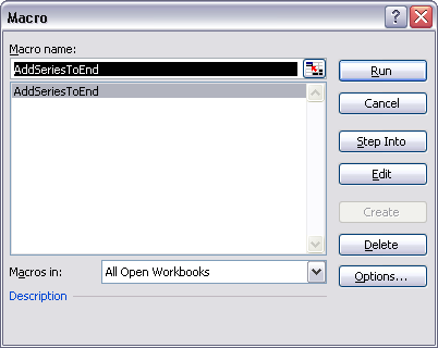
Run the macro: press Alt+F8, select the macro from the list, and click Run.

Here’s the result, which adds the fourth column as the chart’s fourth series.

Naturally, this can be changed using the Source Data dialog, or by dragging the colored outlines that indicate the source data. However, if the existing source data is in a pivot table, the chart would be converted to a pivot chart. Also, if the data is on another worksheet (or multiple worksheets), or if it is discontiguous or even more complicated, this is likely to produce unexpected results, or fail completely.

This procedure only requires that the last series have a series formula that it can parse. The added series is related only to the last series in the chart, using the next row or column in the worksheet.

Here is a chart that initially uses the first three rows of the data range for its three series.

After the macro is run, the chart has four series, using the first four rows of the data range.

Here’s the VBA procedure. If you’re not sure how to implement it, refer to my introductory VBA tutorial, How To: Use Someone Else’s Macro

Sub AddSeriesToEnd()
  '' Add series to active chart
  '' Use same X values
  '' Use Name and Y values one column to right of last existing series
  Dim sFmla As String
  Dim iParen As Long
  Dim sFmlaArgs As String
  Dim vFmlaArgs As Variant
  Dim sMsg As String
  Dim iOffset As Long
  Dim jOffset As Long
  Dim rValues As Range
  Dim rName As Range

  If ActiveChart Is Nothing Then
    sMsg = "Series Formula too complicated to parse"
    GoTo CantHandle
  End If

  With ActiveChart
    sFmla = .SeriesCollection(.SeriesCollection.count).Formula
    iParen = InStr(sFmla, "(")
    sFmlaArgs = Mid$(sFmla, iParen + 1)
    sFmlaArgs = Left$(sFmlaArgs, Len(sFmlaArgs) - 1)
    vFmlaArgs = Split(sFmlaArgs, ",")

    If UBound(vFmlaArgs) + 1 - LBound(vFmlaArgs) <> 4 Then
      sMsg = "Series Formula too complicated to parse"
      GoTo CantHandle
    End If

    On Error Resume Next
    Set rValues = Range(vFmlaArgs(2))
    Set rName = Range(vFmlaArgs(0))
    On Error GoTo 0

    If rValues Is Nothing Then
      sMsg = "Last series values are not in a range"
      GoTo CantHandle
    End If

    If rValues.Rows.count > 1 And rValues.Columns.count = 1 Then
      ' series in columns
      jOffset = 1
    ElseIf rValues.Rows.count = 1 And rValues.Columns.count > 1 Then
      ' series in rows
      iOffset = 1
    Else
      ' one cell or multiple rows and columns
      sMsg = "Series values range cannot be parsed"
      GoTo CantHandle
    End If

    vFmlaArgs(3) = vFmlaArgs(3) + 1
    If Not rName Is Nothing Then
      vFmlaArgs(0) = rName.Offset(iOffset, jOffset).Address(True, True, xlA1, True)
    Else
      vFmlaArgs(0) = "New Series " & vFmlaArgs(3)
    End If
    vFmlaArgs(2) = rValues.Offset(iOffset, jOffset).Address(True, True, xlA1, True)

    sFmlaArgs = Join(vFmlaArgs, ",")
    sFmla = Left$(sFmla, iParen) & sFmlaArgs & ")"
    With .SeriesCollection.NewSeries
      .Formula = sFmla
    End With
  End With

ExitSub:
  Exit Sub

CantHandle:
  MsgBox sMsg, vbCritical + vbOKOnly
  GoTo ExitSub
End Sub