In Using Pivot Table Data for a Chart with a Dual Category Axis, I showed how to make a Chart with a Dual Category Axis using a pivot table to properly arrange the source data. I generally prefer using a regular chart, because pivot charts are pretty inflexible when it comes to formatting. Unfortunately, a regular chart doesn’t know when the pivot table has been resized by a refresh. If you know that the pivot table will only grow in one direction, that is, the number of series remains the same but the number of points in a series may change, you can define dynamic ranges that stretch with the pivot table.
The data initially looks like this:
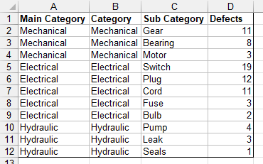
and the pivot table like this, with the top left corner of the pivot table in cell F2:

Let’s define the names according to this table:
| Name | Refers To |
| ‘PT Names’!PTDefectCount | =COUNT(‘PT Names’!$D:$D) |
| ‘PT Names’!PTData | =OFFSET(‘PT Names’!$A$1,0,0,1+’PT Names’!PTDefectCount,4) |
| ‘PT Names’!PTCatList | =’PT Names’!$F$3 |
| ‘PT Names’!PTCat1 | =’PT Names’!$H$3 |
| ‘PT Names’!PTCat2 | =’PT Names’!$I$3 |
| ‘PT Names’!PTCat3 | =’PT Names’!$J$3 |
| ‘PT Names’!PTCategories | =OFFSET(‘PT Names’!PTCatList,1,0,’PT Names’!PTDefectCount,2) |
| ‘PT Names’!PTValues1 | =OFFSET(‘PT Names’!PTCat1,1,0,’PT Names’!PTDefectCount,1) |
| ‘PT Names’!PTValues2 | =OFFSET(‘PT Names’!PTCat2,1,0,’PT Names’!PTDefectCount,1) |
| ‘PT Names’!PTValues3 | =OFFSET(‘PT Names’!PTCat3,1,0,’PT Names’!PTDefectCount,1) |
Note that all names are defined locally for the worksheet containing the data and pivot table. PTDefectCount is the number of rows of data in the original table and in the pivot table. PTData is the data range used as the pivot table’s source. PTCatList is an anchor for the PTCategories name, which in turn encompasses the two columns of main and sub categories, the category labels for the chart. PTCat1 through 3 are the names of the three series in the chart, and the anchors for PTValues 1 through 3, the Y value ranges for the three series.
The chart is constructed like that in Using Pivot Table Data for a Chart with a Dual Category Axis. The three series formulas are:
=SERIES(‘PT Names’!PTCat1,’PT Names’!PTCategories,’PT Names’!PTValues1,1)
=SERIES(‘PT Names’!PTCat2,’PT Names’!PTCategories,’PT Names’!PTValues2,2)
=SERIES(‘PT Names’!PTCat3,’PT Names’!PTCategories,’PT Names’!PTValues3,3)
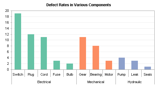
This looks like the previous chart, but it’s now dynamic, ready to change as the data table and its pivot table are updated. Add some rows to the pivot table source data range:
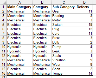
The name PTData expands to include the added rows. Refresh the pivot table:
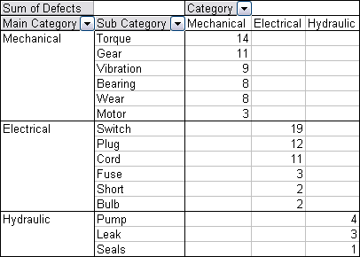
The chart data ranges also expand, and the chart reflects the added data:
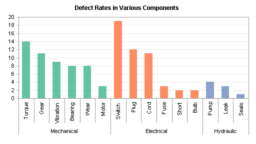
The Mechanical category has moved to the left of Electrical, because its total is now highest. The Category field in the column area of the pivot table has been changed so it is not sorted by defect count. Therefore the series are plotted in the same order (electrical is first), and the colors of the series do not change.
This technique works because I know that the number of columns in the pivot table will not change, only the number of rows. If there is a chance that the number of main categories will change, then this technique will not work, because a dynamic name can only be used to define the X or Y values of a chart series, or its name. A dynamic name cannot be used to specify the number of series in the chart.
Note: In a chart that is not based on a pivot table, a dynamic name can be defined that grows in height and width, and such a name can be used for the chart’s entire source data range (X values, Y values for all series, and all series names). There are two shortcomings with this approach. When you use a name to define the source data range, excel replaces the name by its cell address, and you lose the benefit of having defined a dynamic name. Also, if you define the source data for a chart, and the range includes a pivot table, then the pivot table becomes the data source, and the chart becomes a pivot chart.
Third in a series
- Chart with a Dual Category Axis
- Using Pivot Table Data for a Chart with a Dual Category Axis
- Dynamic Chart using Pivot Table and Range Names
- Dynamic Chart using Pivot Table and VBA


Peder Schmedling says
Shouldn’t it be possible to further develop this method to handle change in number of columns by using some VBA?
This is just a suggestion, I’m not sure if it will work:
Write a class that “hooks” into the events of this chart (that is if it’s an embedded chart, if not just place the code in the code module of the chart), use the Calculate event of the chart to determine when “something changes”. Then use VBA to check if the number of columns changed and and take action if necessary..
Jon Peltier says
Peder – It’s certainly possible, and I show how in the next post.
Eric says
Jon,
Should the last parameter in the ‘PT Names’!PTValues2 & ‘PT Names’!PTValues3 defined name OFFSET formulas be a 1?
i.e. =OFFSET(’PT Names’!PTCat2,1,0,’PT Names’!PTDefectCount,1)
& =OFFSET(’PT Names’!PTCat3,1,0,’PT Names’!PTDefectCount,1)
karthik says
Hi all,
I created a pivot table with some data entered. That’s working fine. But when i change the existing data or create a new entry into the data, the pivot table needs to be updated. Is it possible?
Thanks in advance,
Karthik
Jon Peltier says
Karthik –
You have to manually update the pivot table, or write some code to update it when the data range changes.
Saikat Saha says
Hello Jon,
I have a question for using MTD,YTD on Pivot Tables.
Suppose, I have a sheet that contains data like
Branch A Branch B Branch C
Loan Amount 100 213 757
Now, I want to apply MTD, YTD functions in the sheet so that whenever I would open
the sheet I would get the LoanAmount based on the date like if i open the sheet on 15 August 2010, I would get the Loan Amount from 1st-15th August.
Is there any way to use the above requirement using pivot table. if yes then how. If any more information needed plz. let me know.
Thanks in advance
Jon Peltier says
Hi Saikat –
If the pivot table is grouped by date, you can get YTD grouping by years only, and MTD gouping by months and years, and finding the last value. Of course, any time you group a pivot table, you group the entire pivot cache and therefore any other pivot table linked to that cache. You need to create a new pivot table for each unique grouping, and make sure you don’t save space by using the same source as an existing pivot table
Huzefa says
Hi Jon,
I have been searching your posts on something specific to Pivot tables.
The problem in hand is that I have several columns (static) and rows(dynamic) range of data. I do lots of slicing and dicing of this data using pivot table. The said dataset comes refreshed every week, with the content/status changed of previous dataset and also with new rows added. This info I would want to see in a kind of time based trend analysis, like status changes during last four weeks, improvements occurring during last four weeks, etc. All this has to be refreshed dynamically based on any selection of row or column labels.
Request you send me some in-sights on approach.
Thanx in advance.
Jon Peltier says
Huzefa –
You have to make your code adapt to the changing configuration of the pivot table. If the number of columns in the pivot table does not change, you can use the procedure here without too much modification. If the pivot table changes width, though, you have to figure out how to account for the changes, which named ranges have to refer to which columns, etc. These are custom arrangements very much dependent on each individual situation, and my examples often can only serve as a source of inspiration and ideas.
Fanny Palumbo says
Jon,
the named range solution seems straightforward.
However, it assumes the source data is also in Excel.
Do you have a way to do this when the data is on an external DB?
Jon Peltier says
Fanny –
If the external DB is linked to an Excel query table, my understanding is that the query table behaves like a regular Excel worksheet table. When the query is refreshed, the query table remains intact, and any formulas that reference a column of the table keep referencing the whole column no matter how long or short it gets.
Sobuj says
Great post,
Can you please post a sample worksheet of this? It’ll be really helpful for us to understand
Thanks