Edit Series Formulas - Peltier Tech Charts for Excel

Find and Replace for Series Formulas

The Edit Series Formulas feature works like Find and Replace, but for your charts’ series formulas. For example, you could edit the addresses in these formulas to change the sheet name or the first or last row.

This feature is based on routines described in Change Series Formula – Improved Routines, a tutorial on the Peltier Tech Blog. These routines have been improved and made much more reliable in Peltier Tech Charts for Excel.

Edit Series Formulas in the Peltier Tech Ribbon

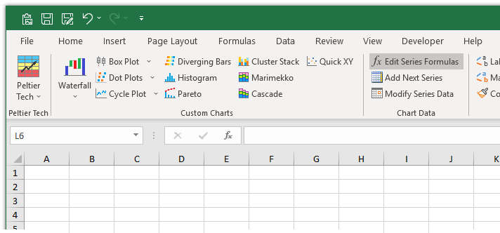
Edit Series Formulas is the first button in the Chart Data section of the Peltier Tech custom ribbon tab. You may select one or more charts, or no charts at all, prior to clicking the button.

Peltier Tech Ribbon - Edit Series Formulas

Edit Series Formulas Dialog

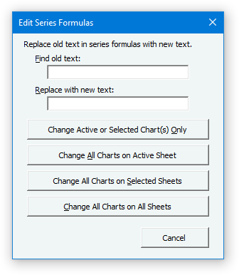
The dialog, shown below, contains a textbox to enter the text you want to search for and replace, and a textbox for the text you want to replace the found text with. There are also one or more buttons, depending on the context of your search. For example, if you select the only chart on the only sheet of the active workbook, the only button will say Change Active Chart Only.

How the Feature Works

The program will cycle through each series of the indicated charts. It will find each instance of the ‘Find’ text and replace it with the ‘Replace with’ text. If Excel disallows a given formula, the replacement will not be made and you will get an error message.

Example

A typical SERIES formula may look like this:

=SERIES(Sheet1!$C$2,Sheet1!$B$3:$B$8,Sheet1!$C$3:$C$8,1)

Within the parentheses there are four arguments, or in the case of a bubble chart, five arguments:

Series name, which can be a cell address like Sheet1!$C$2, text in double quotes like "Series Name", or blank in which case the legend will display a dummy label like Series 1.
X values, which can be a cell address like Sheet1!$B$3:$B$8, an array within curly braces like {1,2,3,4,5} or {"a","b","c","d","e"}, or blank in which case the series will use counting numbers from 1 to the number of points in the series.
Y values, which can be a cell address like Sheet1!$C$3:$C$8, or an array of numbers in curly braces like {1,2,3,4,5}.
The index of the series in the chart (roughly the plot order) which must be a counting number like 1.
Bubble Size, which can be a cell address like Sheet1!$C$3:$C$8, or an array of numbers in curly braces like {1,2,3,4,5}.

I could change series formulas by finding old text Sheet1 and replacing with Sheet2, or by finding old text $C and replacing with $D, or by finding old text $8 and replacing with $10.

Hints

There are several tricks that will make the feature more reliable and easier to use.

‘Find old text’ is case sensitive. Capital C will find column C, but lower case c will not.
‘Replace with new text’ is not case sensitive. Excel will accept a as a new column letter, and automatically capitalize it in the new formula.
To ensure that C only searches for a column letter and not a character in a sheet name, search for $C$ (with leading and trailing dollar signs).
To ensure that 1 only searches for a row number and not a character in a sheet name, search for $1 (with a leading dollar sign).
To search for the first row number in an address, search for $1: (with a trailing colon).
To search for the last row number in an address, search for $10, (with a trailing comma).
‘Replace with new text’ does not need dollar signs matching those in ‘Find old text’. Excel will accept a1 as a replacement for $B$2, and automatically convert it to $A$1 in the new formula.
Entries in ‘Find old text’ and ‘Replace with new text’ will appear in the dialog when called again from the same active workbook.

Documentation Index

Back to Documentation Index