I’ve written about Excel chart error bars in Error Bars in Excel Charts for Classic Excel and in Error Bars in Excel 2007 Charts for New Excel. Both articles contained instructions for adding custom error bar values for individual points, but judging from the emails I receive, a separate article on custom error bars is needed. You cannot add custom error bar values to a single point in a chart. However, you can individual custom error bar values to all points in a plotted series. You need to put all of the individual error bar values into a range of the worksheet. I usually put these values in the same table as the actual X and Y values
Manually Defining Custom Error Bars
Sample Data and Charts
Suppose we have the following data: X and Y values, plus extra columns with positive and negative error bar values for both X and Y directions. The data is set up so that, for example, cells C2 and D2 have the values for the positive and negative horizontal (X) error bars for the point defined by X and Y values in A2 and B2. Cells E2 and F2 have the values for the positive and negative vertical (Y) error bars for this point. The series is plotted using all the data at once, with X in A2:A6 and Y in B2:6. The error bars are also drawn using all the error bar data at once: C2:C6 and D2:D6 for horizontal and E2:E6 and F2:F6 for vertical.

The chart itself is easy: create an XY chart using the data in columns A and B.

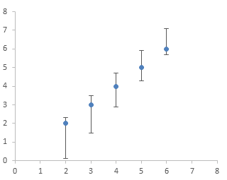
The protocols for adding custom error bars differ between Classic Excel and new Excel. After following the appropriate protocol below, the chart will have custom error bars on each data point, based on the additional columns of data. This chart shows just the Y error bars, to show clearly that each point has custom values different from other points:
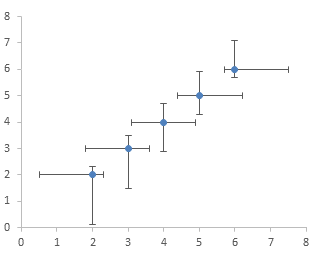
This chart shows the X and Y error bars:
Important Note
A single custom error bar value cannot be added to a single data point, and custom error bar values cannot be added to a series of data points one point at a time. If you select a single value for your custom error bars, this single value will be applied to all points in the series. A whole set of custom error bar values can be added to an entire series in one operation. Put your custom values into a range parallel to your X and Y values as I’ve done with this sample data, then use the manual technique or the utility to add all the values to the chart series in one step.
New Excel (2007 and later)
It is harder to apply error bars in Excel 2007 than in earlier versions. There is no convenient tab on the Format Series dialog. The Error Bar tab(s) as well as the tabs for Data Label, Up/Down Bars, High/Low Lines, and other features have been removed to make them more discoverable, at least that’s what we were told. To discover these features in Excel 2007, select the chart and navigate to the Chart Tools > Layout contextual tab. Click on the Error Bars button, and scratch your head while you try to decipher the options. 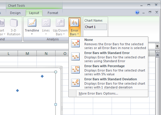 Finally, select the More Error Bars Options at the bottom of the list. X (if it’s an XY chart) and Y error bars with initial constant values of 1 are added to the chart series, with the Y error bars selected, and the Format Error Bars dialog is displayed with the Vertical Error Bars tab showing. (If the chart has more than one series, and you had not specifically selected one series, there is an intermediate dialog asking which series to work with.)
 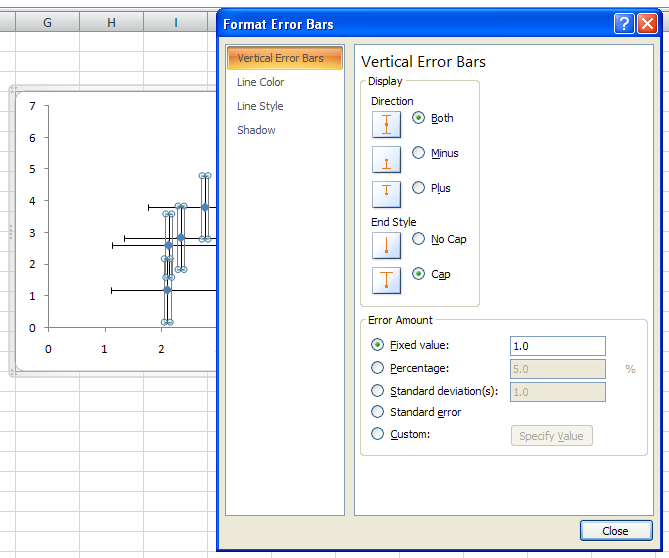 This dialog doesn’t look too unfamiliar. But there is no obvious way to switch to the horizontal error bars. We are used to having two tabs, one for the vertical error bars, and also one for the horizontal error bars. Remember that Microsoft made these chart formatting dialogs non-modal, so you can click on objects behind the dialogs. Click on the horizontal error bars to change the dialog.
 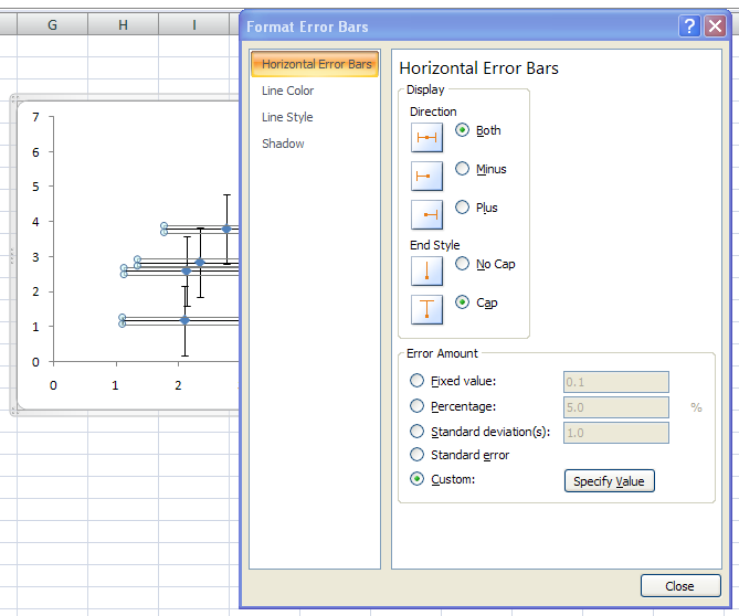 To assign custom values to the error bars, select the horizontal or vertical error bars, and on the Horizontal or Vertical Error Bars tab of the Format Error Bars dialog. Move the dialog so it does not cover the range containing your custom values, then click on the Custom option button, and click on Specify Value. A small child dialog appears with entry boxes for selection of the custom error bar values. (It was easier in 2003, where data entry took place directly on the main dialog, but we’re not talking about productivity today.)
 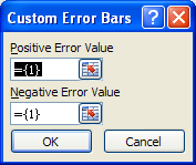 By default, each field contains a one element array with the element value equal to one. You can enter another constant value, and you don’t need to type the equals sign or curly brackets; Excel will insert them. More likely you want to select a range. Make sure you delete the entire contents of the entry box before selecting a range, or at least select it all, or Excel will think you meant to enter something like the following, which will lead to an error message. The edit box is so narrow, that you cannot see the entire expression at once, and it will be difficult to find this error.
={1}+Sheet1!$D$2:$D$6If you want the value to be zero, enter zero. Don’t completely clear an entry box, because Excel will think you simply forgot and it will retain the previous value. 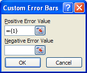
Classic Excel (2003 and earlier)
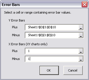
It’s easy to add error bars in Excel 97 through 2003. Bring up the Format Series dialog, by double clicking on the series, by right clicking on the series and choosing Selected Object, by selecting the series and choosing Selected Data Series from the Format menu, or by selecting the series and clicking the shortcut, Ctrl+1 (numeral one). The dialog has a tab for Y Error Bars, and if it’s an XY data series, there is also a tab for X error bars. 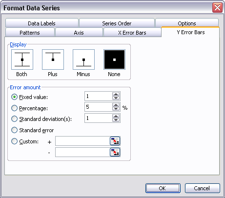 To define custom error bars, click in the + or – data entry box (no need to select the Custom option button, Classic Excel does this automatically), then select the range containing the custom error bar values using your mouse. If you need only one value for all of the points, you can select a single cell, or even type the value you want. This seems redundant, given the Fixed Value option, but this way you can use different positive and negative fixed values or a custom range for one direction and a constant for the other. This is what the dialog looks like with ranges used to define the custom error bar values.
 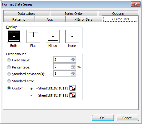 If you want to leave an error bar off the chart, you can leave the data entry box blank.
Notes
The error bars overwhelm the data. To restore the importance of the data itself, use a lighter color for the error bars. Lighten up the axes while you’re at it. 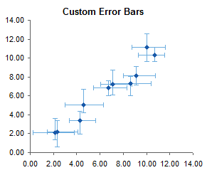 If any custom values are negative, the corresponding error bar will be drawn in the opposite direction: a positive error bar with a negative value will be drawn in the negative direction.
Programmatically Defining Custom Error Bars
The command to add error bars using Excel is:
{Series}.ErrorBar Direction:={xlX or xlY}, Include:=xlBoth, Type:=xlCustom, _
    Amount:={positive values}, MinusValues:={negative values}
Values can be a single numerical value, for example, 1, an comma-separated array of numerical values in curly braces, such as {1,2,3,4}, or a range address in R1C1 notation. For values in Sheet1!$G$2:$G$10, enter the address as Sheet1!R2C7:R10C7. Combine both plus and minus in the same command. In Excel 2007, if you don’t want to show a particular error bar, you must enter a value of zero in this command. In 2003, you can enter a null string “”. In Excel 2003, the range address must begin with an equals sign, =Sheet1!R2C7:R10C7; Excel 2007 accepts the address with or without the equals sign. Single values or arrays may be entered with or without the equals sign in either version of Excel.
Error Bar Utility
To make it easier to use error bars in Excel 2007 (and in Classic Excel), I’ve built a small utility, which you can download and use for free. It’s found in ErrorBars.zip. This zip file contains two versions, ErrorBars.xls for Excel 97 through 2003, and ErrorBars.xlam for Excel 2007. Install this utility by following the instructions in Installing an Excel Add-In or in Installing an Add-In in Excel 2007. In Classic Excel, the utility places a new item, Add Error Bars, at the bottom of the chart series context menu. All you have to do is right click on the series and select Add Error Bars.  Despite all the assurances from Microsoft that context menus work the same in Excel 2007 as in earlier versions, you cannot add an item to an Excel 2007 chart-related context menu. What I’ve done instead is to add an Error Bars item to the end of each of the three Chart Tools contextual ribbon tabs. I know the new philosophy of Office is to place a command in only one place in the whole user interface. I prefer the old style philosophy, however, which is to place the command in every place it may be relevant. I never know where I may be when I want to use a command, and some people remember different hiding places than I do.
 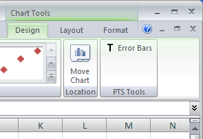 Whether in Excel 2007 or in earlier versions, click on the added command, and the utility behaves the same. Up pops a simple dialog with four data entry boxes, for plus and minus Y error bars, and for plus and minus X error bars.
 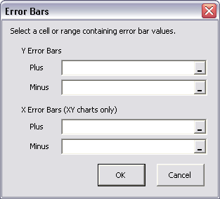 If the chart type is not XY, the X error bar entry boxes are disabled.
 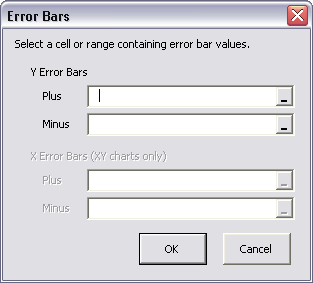 You can select a range or enter a constant into the entry boxes. Leave a box blank to omit the corresponding error bars.
  I hope that this tutorial and the associated utility will make your life easier when working with error bars in Excel 2007.


Michael J. says
You can select the error bar without having to click on it, in excel 2007.
Once the error bars are added to the graph, in the “disposition” tab (Not sure, i have the French version), you can select the error bar you want to edit.
Here’s a pic:
Btw Great tool, as always, thank you for sharing it.
Jon Peltier says
Michael –
Thanks for the reminder that chart elements can be selected from the Chart Elements dropdown, in the Current Selection group, on both the Format and Layout tabs of the Chart Tools contextual ribbon tabs.
Matt Healy says
My personal laptop recently died and its replacement has Office 2010 so now I’m having great fun learning its new interface. It’s like when a grocery store where I’ve been shopping for years decides to rearrange everything: “so WHERE did they move the canned soups now?!”
My wife’s company moved her to Office 2007 a while back, and I vividly remember her expostulations the first time she had to use custom error bars in a graph with Excel 2007! I’m gonna print out and save this clear explanation until I get the hang of Excel 2010.
For me the fun promises to be extended because I’ll switching back and forth between versions as long as my work computer still runs Excel 2003.
drew says
wait a darn tootin’ minute…
the interface is supposed to make the feature more discoverable?
i thought the interface was supposed to help you, not hide things.
wonderful read, thanks a lot.
drew
Jon Peltier says
Hi Drew –
The new interface did a great job of uncluttering the window. However, for me, all that clutter was useful stuff. Hiding important controls merely overburdens my short term memory with tedious navigation details, so I am forced to forget what I was trying to accomplish. The interface designers had no ideas about human cognition or about efficiency and productivity.
Valli says
Thanks so much!
Matt says
Is there a way to display error bars that are specific to each data point? As it is, it seems that the same width of error bars is assigned to all values of a series.
Thanks for this post.
Jon Peltier says
Matt –
That’s the whole point of the article. Follow the steps and use the custom option, then specify a range, so you get the errors that are listed in that range.
Saurabh says
Somehow when I try to add custom vertical error bars, the horizontal bars are added by default and I have given up trying how to get rid of them. They are probably standard error bars. If I go to more error bar options, I dont see a horizontal error bar window. Its the vertical error bar window that always opens. Please help. I need to get this poster printed today. If I try removing error bars, everything goes away.
Jon Peltier says
You need to select the horizontal error bars and press the Delete key. If it’s hard to select the horizontal error bars with the mouse, select another chart feature and use the up/down arrows until the horizontal error bars are selected. Or use the dropdown in the top left of the Chart Tools > Layout or Format tab.
Stuart says
Hi,
I am having the same problem as Matt and cant seem to apply error bars specific to a single data point within a series. I have followed the directions, and when i apply a custom std dev value to a single selected data point, that value is replecated for all the data points in that series. If I try and alter another selected data point within the same series to another std dev value, it again changes the values for the entire series.
Basically, can you have different std deviation values (and hence different error bar values) for several different data points within the same series? If so how?
Cheers Mate
Jon Peltier says
Stuart –
You cannot apply one custom error bar value to one data point. You have to apply a whole range of custom error bar values to a whole series of data points. Put the different standard deviation values for the whole series in the worksheet (a convenient place is in a parallel range adjacent to or near the X and Y values), then use the utility and apply these error bar values to the entire series.
Greg says
And again: how to solve this problem about x-axis labes in bar chart???
I have made a survey, where respondents had to evaluate their agreement with statements (scale from 1-completely disagree to 5-completely agree). I have calculated means and of course, I have made a chart, where vertical axis represents statements, horizontal bars represents values (means)…
now I don’t know how to label x-axis values using text label.
By default, there are labels from 1 to 5 (numbers). I would like to have text labels (“completely disagree”, “disagree”, etc.) instead of numbers (1,2,…). Any suggestion?
Thank you very much.
Greg
ashok says
dear Mr Peltier,
thanks a lot for such wonderful addon, which i liked and found first when i searched in internet. However, why for me only, while adding error bars it says
RUN TIME Error ‘1004’
application defined or object-defined error
from microsoft visual basic editor window and without anything happening.
if there is a solution to it i would be very helpful.
i run excel 2007 in vista.
Jon Peltier says
Hi Ashok –
What were you doing just before the error occurred? Had you selected a series then clicked the button on the ribbon? Or had you tried selecting data for the error bars?
Is your Excel 2007 updated to Service Pack 2?
ashok says
Dear Jon,
thanks a lot for your thoughtful insight. yes, i did not have EXCEL sp2 installed. after that installation everything is clear.
and another stuff to note:
if I select the whole graph, nothing happens.
if i select the bars, then only it works. Obvious though.
it is highly simple and effective.
thanks again.
lenore says
Hi,
Thanks for the useful site. I would like to add different standard error values to different sections of my line graph. Do you know how to do this? I understand I can choose the custom option and then select ranges of values for the positive and negative standard error. But excel doesn’t seem to know what sections of my line graph I would like to apply each error bar, and that I don’t want one for every point, just specific ones. Any suggestsions?
Thanks,
Lenore
Jon Peltier says
Set up your custom range, with one value per data point. Put the value you want in the cell corresponding to each point, leaving blanks where you do not want an error bar. Follow the protocol for adding custom error bars to your data using this range of values.
Lenore says
Thanks for the response Jon Peltier, that is helpful. One more question. I calculated standard error for each data point as you suggest. But excel asks for a “positive error value” and a “negative error value”. I find this confusing because I calculated only one standard error of the mean value for each data point (calculated as the standard deviation of my repetitions/square root of my number of repetitions). So why is excel asking for two values? For example if I calculated 4 for my standard error should I put 2 on either side of my data point or 4 on either side as the “positive” and “negative” values?
Thanks very much,
Lenore
Jon Peltier says
Lenore –
Excel asks for positive and negative values because they need not be the same. There may be an asymmetric error, or you may want to show a deviation only in one direction.
If you have calculated an error value, use that value for both positive and negative error bar values. In other words, for custom error bars, use the same range for positive and negative error bars.
Lenore says
Thank you!
Lenore says
Hello Jon,
As you suggested I make a column of standard error values next to my data columns that I plotted. I left a blank where I did not want a standard error bar plotted (I also tried leaving a 0 with the same result). However then it plots the horizontal standard error bars that I want, but for the ones that I left blank it plots a short horizontal line with no line “cap”. I know you suggested leaving a blank at the data values I don’t want error bars for, however it seems to be still plotting a line there. Any suggestions?
Thanks very much,
Lenore
Jon Peltier says
Lenore –
I think what you’re seeing is not a short horizontal error bar with no end cap. I think it’s a zero-length vertical error bar with horizontal end caps, and it’s these end caps you think are short error bars. This is one of the things about error bars in 2007 which is a little frustrating. Try a blank in the cells for the vertical error bar values.
louise says
Hi Jon,
Thanks for the explanation of error bars! It really helped, I seem to be having the same problem as Lenore,
I have managed to get the error bar correctly assigned to each point within the series by adding the column parallel but my positive and negative values are the same and it wont allow me to enter the same value for my negative as for my positive,
A dialog box pops up saying the formula I have entered contains an error so basically i only get an error bar above the column on the graph, wondering if you can help
Jon Peltier says
Louise –
What is the formula you’re entering? Are you using the built-in custom error bar value dialog, or the error bar utility I’ve written? If it’s the built-in one, are you sure there it doesn’t begin with the leftover “={1}+”
Tri says
Dear Jon,
Thank you so much for your useful explanation and tips.
I got problem with inserting error bars one by one as you said, and I tried to install your utility, but it displays something “Visual Basic error” and also requests a password.
Do you have solution for these?
Thank you in advance
Researcher says
Hi Jon,
Thanks a bunch for this helpful tutorial!
Ed says
Thank you! Thank you! Thank you~!! Excel 2007 is a pain in ass when it comes to error bars. I do lots of custom stats analysis and even something simple as putting std dev bars on scatter plots is insane in default settings. Your utility is a must have!
Jaime says
Thank you so much…u saved me…. :D
Danièle says
Well, I am using only custom error bars, so my questions is more about the standard choices excel gives?
I am still suing excel 2003 for work, and someone complained about my using custom error bars whereby I calculate the std errors for each data point, and place then in a separate column, and use that range for my custom error bars. I was told that I should just click on the data, and choose the standard error bar option, and excl would automatically add them. How would excel know where the original data from which I averaged the data values, and to which I am adding the error bars comes from? I have been searching, but there are no real explanation as to how excel manages to guess the standard deviation or the standard error!
As always, each time I read the blog, I am amazed by excel, but not with the error bars…
Thanks!
Danièle
Jon Peltier says
If you use the built-in standard deviation, Excel uses the standard deviation of the values plotted, centering the error bars on the average of the values plotted. Looks ridiculous, but maybe it’s easier for some people than using a horizontal line at, say, ±3 stdev.
If you use the built-in standard error option, Excel calculates the standard error (standard deviation divided by mean) of the plotted values, and plots this same value for each point.
Neither of these options provides custom error bar values for each data point.
Danièle says
I always wondered how excel could ‘guess” what you wnated, or at least “guess” where to get the data from! Now I know!
Thanks!
Chris says
Hi Jon,
I have Excel 2010, and I’m trying to create a macro that graphs the relationship of two columns of data in a scatter plot. Everything works fine until I try to get the macro to record my use of “Format Error Bars” for custom amounts. Specifically, I want each data point in the set to have a vertical positive and negative error bar that corresponds to the values in the third column of my original chart (same values for positive as for negative). I don’t need any horizontal error bars. Do you know of a way that I could make this macro-compatible?
The error in the code is listed as:
ActiveChart.SeriesCollection(1).ErrorBar Direction:=xlY, Include:=xlBoth, _
Type:=xlCustom, Amount:=0
Thanks for your time.
Jon Peltier says
Chris –
If you scroll down, you’ll see where I included the syntax for adding error bars:
You need to include both positive and negative error bar values, as a constant (if they are all the same, a comma-separated array of numerical values in curly braces (such as {1,2,3,4}), or a range address in R1C1 notation.
Chris says
Thanks a lot Jon! Your advice was extremely helpful.
bill says
Thanks for this blog topic and comments!
helmer says
I have read your very helpful article – thank you for your work on this !!
I have followed the steps ( doing the worksheet layout as you depicted) and it works -but I have one problem :
– The y-value error bars are associated with y-values in numerical order. Say you have y-values Y1, Y2, Y3. The appropriate error values are depicted in numerical order from the largest to the lowest error value, attached to Y1. Y2. Y3 respectively.
How do I remedy this ?
Thank you very much for your time and effort.
helmer says
above comment edited :
The problem was that error bars are depicted numerically by default.
The error bars are not associated with the appropriate Y-values.
I did the worksheet entirely as you described, using x and y values, error values both positive and negative. However, my X values are names and not numbers.
rohini wankhade says
thank you
mahraz says
Hi,
I installed the add in on excel 2007, however, still, the error bar adds to ALL of my points on the graph, is there any way to stop this? I need to add different error bars to different points on my graph.
Jon Peltier says
Mahraz –
Error bar values re assigned one series at a time, not one point at a time. This means you have to put the error bar values into a worksheet range, then select this range in the utility (or in the regular dialog).
mahraz says
So do I do what you have done on the top of this page with the Y err +, Y err – ?
I am doing a scatter graph and I have three points. I need to assign three different ranges to each point…I have spent a lot of time on this, I still don’t really understand how to do this.
I would really appreciate it if you could please explain a bit more? like a step by step process?
thank you!
Jon Peltier says
Mahraz –
Yes, you have to set up your data like my example at the top. Use my dialog to enter the data in columns C, D, E, and F for the selected series.
mahraz says
I only have Y err + and Y err -. I have added these, and I have a graph for my X and Y column values… but when I highlight X, Y, Y err + and Y err -, and then graph, no error bars show up and my scatter graph looks a bit weid….
When I have my X Y graph, what do I do from there to add the Yerr + and Y err – as error ranges?
sorry if i’m asking the same question over again….im veryyyy confused.
Jon Peltier says
As the article states, you have to make your chart using the X and Y data (in columns A and B in the example). Then you add the error bars, using the built-in interface or using the utility I’ve provided.
Robert says
Hello Jon.
Thank you very much for this blog-it assisted me in dealing with issues regarding placing error bars of separate data points in a series using Excel from Office 2010.
In turn, I thought I could constructively critique one of your posts mentioned above. You mentioned that Excel calculates the error bar by dividing the standard deviation by the mean. I would like to offer a correction to this: the standard error is typically calculated by dividing the standard deviation by the square root of the sample size. I am assuming this is how Excel automatically calculates the value for the error bars.
I always calculate my error bars and manually enter the values when I add them to Excel-made graphs. Please correct me if I’m wrong about the automatic calculation of the error bars within Excel, as I know many other scientists who use Excel to express their standard error of the mean values using this error bar option.
Thank you!
Jon Peltier says
Robert –
You’re right about the standard error.
I don’t know what I was thinking, but I’ll update those other posts.I can’t find the post where I misstated the definition of the standard error; do you recall which article it was? Thanks for the heads up.Daniel Elder says
Jon,
I cant find a way to put error bars in that change from data point to data point..pls help
Jon Peltier says
Daniel –
Did you put the individual error bar values into a range of cells? Did you use the Custom option to define the error bar values? Did you select the entire range of error bar values that you entered into the worksheet? What value do the error bars have, if not the range of different values?
Kathy says
I’m having the same problem as many others who’ve commented. My data are formatted as you explain with my SE series in a corresponding range. I enter the SE range as described in your instructions for custom error bars. I get error bars but they are not at all the values in the range. It seems like Excel is selecting the major unit value from the y-axis.
I can’t tell from reading the comments if people actually fixed this problem after reading your response or if they gave up as I’m about to.
Also, I downloaded your add-on utility and installed it. It shows on the chart options tabs but nothing opens when I click on it. I have Office 2010.
I have benefitted many times from your posts and hope you’ll be able to help on this one, as well. Thank you.
Jon Peltier says
Kathy –
You have to select “Custom”, then select the ranges in the dialog, then not select a different option.
When using the Error Bar Utility, you have to select the series that you want to add error bars to, then click the button on the ribbon. Without selecting a series, the utility doesn’t know where to add the error bars, so it bails out.
Sue E says
This issue has been brought up before but I still don’t understand the answer! My problems is with applying separate error bars within a series. You state above:
“A single custom error bar value cannot be added to a single data point, and custom error bar values cannot be added to a series of data points one point at a time. If you select a single value for your custom error bars, this single value will be applied to all points in the series.”
If there is no way to apply a separate error bar to each data point with in a series, are my only options are to create single data points so there are no series (which I’m not sure how to do) or find a earlier version of Excel? I am edited a graph I created in an early version of Excel where I could apply different error bars to different data points within a series.
Thanks so much for your help. Your instructions on Excel are the best out there!
Jon Peltier says
Sue –
The very next paragraph begins “A whole set of custom error bar values can be added to an entire series in one operation.” It then describes how to put custom (different) error bar values onto a series of data points.
Sue E says
Jon-
FINALLY figured it out. Sorry for not reading carefully enough! Thanks for your help.
Sue
Kathy says
Jon, I am so excited to add real error bars to my graphs. I followed your instructions, and everything worked perfectly until I actually tried to use it, and then I am asked for a password!
What do I do now?
Jon Peltier says
Kathy –
The password prompt happens because some add-in (not mine) is misbehaving. It isn’t even always an add-in for Excel. The prompt usually does not interfere with operation of my program, only with closing Excel, and you just need to click Cancel. When I have a chance I’ll write an article about what causes it and how to get around it.
RobH says
Thanks for this. Excel 2010 doesn’t half make it hard to put the standard error on a graph. What is particularly dangerous is that the default value it puts on a summary graph (e.g. a column chart, which is when you are most likely to want to use a standard error) is completely invalid (I presume the default it is the standard error between the different summary datapoints). Also to define the values to use with the custom standard error you have to select ‘specify value’ (rather than values) which suggests that you can only select on value for the entire series, which is where I think some others have understandably got confused.
Mike Ritchie says
Jon
Simple request. I want to put 95% confidence limits around some bar chart means. I cannot believe excel (2007) needs me to calculate the Confidence Limits in separate columns in order to then plot them. Is there no excel add in that provides a drop down tool for CL’s in the same way as it automatically plots 5%, SE, SD around the means? It is only a small step to plotting CL’s automatically. Surely it can be automated? What am I missing?
Jon Peltier says
Every branch of statistics must have its favorite way to indicate some kind of largest acceptable or largest expected deviation from its favorite calculated middle. If Microsoft tried to include them all, development in other areas would grind to a halt. Sure, 95% CI seems common enough, but they had to draw the line somewhere.
Personally, I prefer to calculate my own error bar values. Any parameters entrusted to Excel come from a black box. I can look in the column of cells to make sure it’s doing what I expect. Of course these things could be automated, and probably they have, but I don’t know of a specific place you could look.
Carole says
Very helpful! Thanks!
Back Tomas says
Most helpful, Thanks a million!
Graham Whalley says
Hi Jon, I have spent many an hour reading books in the library and Computer outlets ,looking for some mention about Error bars and how to progress from the custom button. But to no avail . Why didn’t I look on Google and your Blog, who knows ? It was so good to be part of a community . Although by the time I had read the complete thread I was a little overwhelmed. Onwards into an uneasy future. Best regards Graham.
Geoff W says
Jon, thanks for the Excel 2007 Error Bar utility tool. After reading your detailed description of options, this was the only way I found to add horizontal error bars to a particular series on a simple Excel 2007 chart.
Richard Lohaus says
Thank you for your clear explanation which helped solve my problem!
Claire Gummerson says
Hi,
I’ve read this page over and over again but still can’t solve my problem (and unfortunately can’t download you’re tool either because its blocked here at work). I’m having the same problem as Sue E – I’ve got a column of my values, the next colum of the lower confidence interval value, and the next column of the upper.
I go to custom, specify value and highlight the relavent columns as a range in the ‘positive error value’ and the ‘negative error value’. But Excel still doesn’t seem to use these and i end up with a wide confidence interval on each point that goes into the negative (even though none of my confidence interval values do). Please help, i have read the page over and over again, but somehow still can’t figure it out. I’m working in Excel 2007 by the way. Thanks.
Jon Peltier says
Claire –
You need to enter the values that represent the lengths of the error bars, not the values at the ends of the error bars. That is, half the width of the intervals, not the upper and lower values the mark the boundaries of the confidence intervals.
Claire Gummerson says
Ahhh i see. Thanks so much for your quick response.
Sam R says
Thank you so much for this. I have just spent an hour and a half trying to do this with no success. I even tried to do it in R (with no success) because I was getting so annoyed with Excel! With your article it took me two minutes. You are a life/time saver!
Evan Jones says
I have been horribly frustrated. I want to get ONE error bar for ONE bar which is the average of a series of data points.
I have, say 10 bars. Each bar is an average of a separate column of data. (So, 10 bars, 10 columns of data. I want 10 different error bars: for each set of elements that make up each bar.)
But when I drop in an error bar instead all I get is the error bar for the value of all the columns in the same series. And each bar is counted as a single data point (how useless is THAT?). If I make each bar a separate series, I get no error bar at all; (it’s treating it as if I had only 1 data point even though the single bar is an average of a whole bunch of different data points — for which I want the standard error.)
My very lengthy and very clumsy workaround is to:
A.) Make every bar a separate data series (ick).
B.) Independently calculate the error bar using =STDEV(Data Series)/SQRT(COUNT(Data Series)) for (Standard Error) for each and every miserable data series that makes up each and every bar. (Around 3000 bars of data — so far . . .)
C.) Manually cut/pasting each and every result in each and every bar of data (double-ick).
Not only does this take forever+1, but it is prone to the usual cacophony of cut/paste errors and typos. And the paper my sheets are supporting is going into the teeth of the most implacable, virulently hostile peer review this side of Hell. If I don’t get it RIGHT, they are going to dangle me by my toesies — and that’s just my co-authors.
There has GOT to be a better way! Right? Right . . . ? RIGHT?
Peter says
Great article, thanks Jon! Aside from the ribbon itself, MS have done an abysmal job with custom error bars (hence my stumbling on your article) and in Excel2010 it seems to have some bugs. Minor annoyance is the default ={1} does not get replaced with range selection, so that seems to first need to be deleted. More significant is that sometimes it won’t take a custom range at all (stays stuck on default/won’t accept custom range), and does not seem to display the new range once entered so is not simply manually editable?! Maybe it doesn’t like my range, but I don’t see why it shouldn’t and there is no feedback/error trapping. Maybe we should all roll-back to 2003. I liked it so much better and still regret the ‘up’grade.
Jon Peltier says
Evan –
I hope the 3000 bars are not all on the one chart!
So in your example, you have 10 columns of data. Put the bar category labels in A1:J1.
Put the data into A:J starting in row 4. So if there are 25 points in each, this will fill A4:J28.
Put the average calculations (which you are plotting) in A2:J2.
Put the error bar calculations in A3:J3.
Make a bar chart using A1:J2.
Using the approach outlined in this article, add custom error bars to the data, using the range A3:J3 for both positive and negative error bars.
Evan Jones says
Thanks for your reply. I will figure out your suggestion and try it out and let you know how I fare.
(The 3000 bars are all in one workbook, spread over ten separate spreadsheets. 10 charts per sheet, 30 bars per graph.)
frank says
Jon,
I wonder whether you or someone else having the same issue that I have on Custom Error Bar on Excel 2010. I can only specify value on the Custom Error Bar and I can not specify a cell reference at all(like =Sheet1!$A$1, which I can do that on Excel 2003!
My excel 2003 using cell reference like Sheet1!$A$1 will work correctly when open with Excel 2010 but I just can not modify it any more unless I am in Excel 2003(and I am going to lost access to Excel 2003 very soon).
Using VBA inside Excel 2010 or using VBScript to modify the Custom Error Bar field will give me error just like other fields that won’t allow formula or cell reference.
Just wonder whether you or anyone else having the same issue and know any work around(or MS certain patch fixing the issue)? Thanks!
Jon Peltier says
You have to make sure to delete the contents of the range entry boxes. Even though they are totally selected, when you select a range, the range is appended to the box contents. The default is
={1}
If you don’t clear the box, but just select Sheet1!$A$1, the box now contains
={1}+Sheet1!$A$1
which is illegal. But because they made the dialog so infuriatingly small, you can’t even see all of “Sheet1!$A$1” at once.
Peter Lancashire says
I have installed the add-in into Excel 2010. It works fine. Thanks. The buttons appear in the ribbon only for standard charts, not for PivotCharts. If you are updating the add-in, a nice addition would be a way to step through all the series in the chart in the dialog box itself.
Jon Peltier says
Peter –
The buttons appear on the Chart tools tabs, but I neglected to also put them onto the Pivot Chart tabs.
I’m thinking about adding the Error Bar tool to my utility. It will be available for any chart, and a series selection dropdown on the dialog would certainly make it easier to add error bars to multiple series.
cp says
Great article. I am plotting the 95% CIs around odds ratios. I am able to do this by selecting the range of values that comprise the upper and lower limits. However, the error bars are not reflective of the numbers on the Y axis. For example, I have an OR = 1.06 with a Lower Limit if .50 and upper limit of 2.28. The bar looks like it ranges from .75 to 3.75. Any ideas on this?
Jon Peltier says
The values used for the error bars are the lengths of the error bars, not the values at the endpoints of the error bars.
cp says
Thank you! I just needed to compute the differences and it worked great.
Rachel Breyta says
Hallo-
I’m having the same problem as mentioned by Matt and Stuart, and I have applied the custom error values in series as you instructed. What I get are error whiskers who’s values do not seem correct- higher or lower by anywhere from 50-500 units. when I check which cells are supplying those values, they are correct, and entered in the same order as the original data points. I cannot find a pattern that would indicate that and error like error values for series c being applied to series d, for example. this is so frustrating
Jon Peltier says
Rachel –
Matt and Stuart were trying to add error bars to a single point, not to an entire series.
Are you using the desired lengths of the error bars for your custom values? Are you adding the error bars to the corresponding series?
Kendal says
Is there any way to remove the brackets that appear at then end of error lines? It’s some what annoying having to increase the size of my data points to cover those lines.
Jon Peltier says
Kendal –
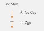
Format the error bars, and select the option without end caps:
Guus van Zuylen says
Hi Jon,
This looks like an awsome utility.
However, after installation under Excel 2013 I do’nt see it at the right hand side of “Move Chert Location”.
In VBA I see the project PTSErrorBars, a password is required.
Thanks,
Guus
Jon Peltier says
Guus –
I’d noticed that once before, but never really looked at it. But I checked it out today, and thanks to a little help from my old colleague Ron de Bruin, it’s now appearing in Excel 2013. Delete the old version and download it again.
By the way, you don’t need the password to use the utility.
Kay says
i would just like to say thank you. Having started with a dos package called FigP and gone through early excel I have been boring family and friends about how putting custom error bars on charts has became an increasingly embedded feature from whatever version of excel it was (2007?). Have been through 2010 it was just as difficult but at least largely unchanged. I have just got 2013 and its no easier and there is the usual moving the feature to a different tab just for a bit of fun. BUT downloaded your utility and you have answered all my dream, its easy now!
Thank you again
Mark P says
Jon, too bad your Utility does not work on a MAC – I tried to install it and gave me an error about iy having a macro.
I am racking my brain here…
Great Tutorial though!
Jon Peltier says
Mark –
What was the exact error message? I’ve never tested that add-in on a Mac, but I don’t know offhand what would make it fail. If you’re installing the file as an add-in, it shouldn’t warn you that it has macros, because add-ins need code to work.
Mark P says
Jon, I tried both files (xla and xlam) – here is the error message – http://www.primaveraphoto.com/Add-in-error-for%20mac.png
Mark P says
Up in Error Bar Utility – the links give a 404 error
“Installing an Excel Add-In or in Installing an Add-In in Excel 2007.”
I got Excel running on my virtual machine and went to install the Error Bar Utility and it asked for password?
Almost have it working :)
Jon Peltier says
Mark –
What version of Office for Mac are you using? VBA worked in 2004, and works in 2011, but Microsoft suspended VBA support in Office 2008. This message looks like it relates to Office 2008.
If you are using 2011, was VBA not activated when Office was installed?
Jon Peltier says
What else is installed for Excel on your VM? You don’t need a password, but sometimes interference with other add-ins and third party programs makes VBA think it needs access to the VB project of my add-in in order to shut down Excel properly. It’s a spurious message which Microsoft has given us developers no means to address.
Mark P says
Jon, I sent you an email earlier – I went to my office and tried your add-on in the new Excel – It worked out but now cannot get custom error bars for each point. Please refer to the file I sent you via email.
I am not too worried about getting it to run on my home VM, but when I did use it I received the following error http://www.primaveraphoto.com/compile-error.png
Like I say I am not too worried about getting it to run at home.
Mark
Jon Peltier says
Mark –
Which add-in gave you this error (xla or xlam)? I haven’t tried either in Excel 2000; I don’t think I even have 2000 any more. The xlam freshly downloaded from the blog has just worked for me without issue in Excel 2010.
KC says
Hi Jon
Can we use range name as Error Value please?
Does not seem to be able to in my Excel 2007.
KC
Jon Peltier says
KC –
I just tested in 2010 (I don’t have 2007 on this machine). I named a range “plus” for the positive error bar values and “minus” for the negative values. I applied error bars to a set of data, added error bars, then formatted the error bars to use custom values. I tried entering the Names in the dialog (e.g., “=plus” and “=minus”), but that did not work. I had to prefix the sheet name in front of the Name, that is, I needed to use
=Sheet1!plus
=Sheet1!minus
for the references to the positive and negative error bar values. With this minor modification, it worked fine.
KC says
Hi Jon
Thank you. I just want to confirm it works.
I should kick myself for clearing one of the value boxes, causing Excel to retain previous value.
Problem solved please.
Liz K says
Hi Jon,
Apologies if this is an obvious fix, but here’s my problem: I can add custom error bars to my data series just fine (I have a bar graph with 6 bars on it, paired into 3 major categories each), but the error bars for the last two bars (both in the last/third category) don’t show up–all I get is a little selection dot over the top of each graphed bar ( the bars representing a data set), but no actual error bars. How can this be happening, when my SEMs do NOT equal zero and I’m inputting the values as directed–the error bars work for the other data, after all? I am working in Excel 2013.
Thank you for your help!
Jon Peltier says
Liz –
If you post the workbook (e.g., Dropbox) I can take a peek.
Sancho S says
Hi Jon,
Is it possible to programmatically get the ranges used for error bars (not set them)?
Thanks a lot!
Jon Peltier says
Sancho –
This isn’t exposed to VBA. I’ve thought about trying the dreaded “SendKeys” to select the comments of the input ranges in the dialog, then copy and extract the comments if the clipboard. But such thoughts less to migraines.
Sancho S says
Thank you Jon!
I would face the SendKeys way only if benefiting significantly from such automation.
BTW, did you ever use SendKeys for “similar” purposes? Is it expected to succeed?
Thanks
Jon Peltier says
Well, knowledge of the ranges used for custom error bars would be a significant benefit. But SendKeys is a significant source of pain.
Ah says
how to calculate positive and negative value of standard error bar excel?
Jon Peltier says
Standard error is standard deviation divided by square root of sample size.
Jms says
Dear Jon Peltier
I am trying to set just Yerror bars but it shows Xerror bars also. What I did, I have some data which are, I put them to be, Yerror bars. Then from Format Error Bars—–> Vertical Error Bars—–> and then click on Custem —–>Specify Values and for both negative and positive values I import those data but I got both X and Y error bars! Is this correct what I have done it or not? If not could you please tell how?
May thanks in advance.
Best wishes,
Jms
Jon Peltier says
When you add error bars to an XY Scatter chart, Excel adds both vertical and horizontal error bars. Simply select and delete the ones you don’t want.
Jms says
Thanks for kind reply. To be honest I did that before posting my question but the problem when I check the Format Error Bars again I see the Error Amount changed frorm Custom to Fixed value which I do not want that. Any clue please?
Best wishes,
Jms
Jon Peltier says
Jms –
You didn’t do anything to make Excel think you were adding the error bars back from scratch? The whole Error Bar experience in Excel is a bit mystical.
coolBlue says
Hi, Thanks for the insights Jon, sometimes it seems like more and more features in excel are cowering in the shadows, hoping not to be noticed (I guess MS quite sensible, wants to manage their code base), so its really great that you generously share your knowledge like this.
I saw a few questions about how to create individualized error bars that are different for points in the same series. The need for that is what brought me to this page. I notice you make a definitive statement that it is not possible to access and format individual error bar objects, which is really refreshing. So often I see answers that avoid the question and just offer a work around… but not here! Kudos for that.
I would add that the work-around I found was to write some code to break the series into groups of points sharing the same characteristic that determine the error bar format and add a separate series for each group. Then you can format the EBs for each group to get the desired effect. In my case I don’t need a line so its quite straight forward. If a line is required, I guess you could just leave the original series there undecorated and superimpose the auxiliary series (serieses, seris??).
Cheers!
Jon Peltier says
Cool Blue –
Leave the original line undecorated, and superimpose auxiliary series. Exactly. This is how to think outside of the Excel box.
Alex Hannon says
Thank you.
Your explanation of error bars in Excel is truly helpful.
Hakeem Niyas says
Dear John
I have validating my numerical values with the experimental data. Both have a close match.
The experimental error is +/- 2%
I tried to put an error bar to my experimental results and show that my numerical results are well within the experimental error bars
I have about 250 data (1 data per min)
I have put an error bar – But the entire graph becomes dark and filled with error bar
As my error bar value is constant, I just want to put few (1 for 10 data – 25 ) error bars which will not hide/dark the graph
Is there any way to do this?
Thanks
Jon Peltier says
Hakim –
The easiest way to put error bars on only some of your data is to add a new series that contains only some of your data, hide these new points (format with no lines and no markers), and put error bars on these hidden points.
Prince says
Hi, please I would like to know why the size of a bar chart changes when the error bar is inserted, and which size to use when interpreting the result (the one before inserting the error bar or the one after inserting the error bar?)
Prince
Jon Peltier says
Do the bars change size? Do they become shorter to allow room for the error bars? Bar charts are not ideal for error bars, since the minus error bar may not appear clearly against the bar itself.
Prince says
Hi Peltier, Thanks for you response, sorry i couldnt get back before now. the error bars cause change in the length of the bar charts. Also I would like to know, when comparing data using the error bar, what is the implication of the difference in length of the positive and negative error bars?
Jon Peltier says
1. The bars don’t unilaterally change length. The axis scale also changes to match the change in the bars.
2. If the positive and negative error bars have unequal lengths, it means that the quantities you are representing with error bars are unequal. You need to think about what the error bar values mean.
Prince says
Thanks Peltier, I think this would do, I appreciate your help/
Ola Fincke says
I have been doing bar graphs in excel a lot. All of the error bars work except for the last bar in one set of three. It sets the error bars correctly for the first two, but will not put any on the third, even though I have the s.e. filled in the box, just like all the others. Each box is divided into 3 sections. The last one has only 2 sections because the value for one is ‘0’. I thought that might be the problem, but even when I put in fake data so there are 3 boxes, it still won’t put an error bar on the 3rd box. What gives? I have to get it right because my paper was accepted, and I manually created an error bar but now that it’s going to be published, I need all the error bars to be the standard ones. Thanks for any help you can offer!
Jon Peltier says
I don’t understand your description of the data or the chart. Do you have a link to your file?
louisville plumbers says
When I initially left a comment I appear to have clicked on the -Notify me when new comments are added- checkbox
and now whenever a comment is added I receive four emails with the same
comment. Perhaps there is an easy method you can remove me from that service?
Thanks!
Jon Peltier says
I wish there were an easy way to track all the people who have subscribed to messages. I can see a large number of them in one WordPress plugin, but your email address wasn’t listed. There’s another source of email notifications, through feedburner. I can see the subscribers to the feedburner email service for blog posts, but not for comments, which must be what you’ve signed up for. Sorry.
Vikrant Saini says
I added the excel utility errorbar.zip and installed the add in. the button apears in Chart-Design ribbon but does not respond when i click the button.
Ed says
Hey Jon,
Saw this discussion and hoping you can help!
Maybe you have mentioned this, but I am having an issue when transposing the graph that already includes error bars (the error doesnt transpose). Currently I have it setup such that it graphs the rows on the x axis and columns on the y (I assume the default setting). My error is also in columns such that when I go to “custom error bars” I can easily add the positive and negative error by just dragging down the column. The problem is that I would like the data presented with the columns on the x axis, and the rows on the y axis (ie. transposed). When I use the switch rows/columns option under select data on the graph, it does transpose the graph, but the error bars disappear? Any idea how to keep them included?
It is way too time consuming to try and add error bars by row, mainly because I cannot drag straight across the row. Moreover, there are 100s of row, but only 5 or 6 columns.
Thoughts?
Ed
Jon Peltier says
When you switch rows and columns, Excel only switches the X and Y values. Error bars are at least one level removed from that, and are not included in anything that can be switched.
Nandini Kar says
Hi Jon,
I am using the Mac office 2011 and it makes the custom error bars without any issue. However, even though I specified the same data series for both positive and negative, somehow some of my data points are showing different error (i.e. the bar length is longer in positive or in negative side).
I was wondering if this ever happened and how to fix this.
Thanks,
Jon Peltier says
I’ve never known this to happen, unless the axis scale is logarithmic, so a delta X would result in longer error bars on the low side of the points.
Frank Krumm says
Hi John,
your article is the only one I find approximating my problem. I’m trying to set up a chart in vbscript and setting the ErrorBar keeps me busy. I tried almost everything besides sendkeys to put the values in.
I always get an error message: “zerlege_UC.vbs(585, 8) Laufzeitfehler in Microsoft VBScript: Unbekannter Laufzeitfehler” (translates to “unknown runtime error”)
Here is the line in the vbscript:
oExcel.ActiveChart.SeriesCollection(1).ErrorBar xlY, xlMinusValues, xlCustom, , “=R2C14:R” & sheetNumber & “C14”
sheetNumber is 20 when runtime error occurs, all constants are set.
Do you have an idea why I get this runtime error?
bye
frank
Gladys says
Hey there!
Is there any way for me to add horizontal error bars in a pivot chart? I’m using excel 2010…
Thanks!
Jon Peltier says
Gladys –
Horizontal error bars are only allowed for XY chart series (or horizontal bar charts, which is unlikely to help), but pivot charts do not support XY chart series.
Marc Goodrich says
Hi Jon,
Thanks for all of the advice on creating custom error bars! I was able to create custom error bars for my figure in Excel 2016, but have had the same problem as a couple other commenters that the bars for the last data points in a series do not appear properly (either half or none of the error bar appears), despite having data entered in the appropriate cells. I noticed that when other people had these issues you asked for a link to the file, so I have sent the file via dropbox. I would greatly appreciate any advice you have for fixing this issue, as I have tried everything I can think of and nothing seems to work. Please let me know if you have any trouble accessing the file.
Thanks,
Marc Goodrich
Jon Peltier says
Marc –
I’ve recreated your example below, simplifying the labels and multiplying the error bar values by 4 so they show up more easily.
If you think about it, while you have six values and six errors for each series, you are plotting eight points for each series, including the gaps between A2 and B1 and between B2 and C1. Some of the errors are applied to these gaps, and since there are no values, there are no bars on which to anshor the error bars.
It is always best to put the errors in parallel ranges, so you can ensure that the appropriate error values line up with the appropriate data values. If I transpose the error values and place them next to the data values, it’s easy to see what is wrong. The ranges containing error values are six rows high, while the ranges containing data values are eight rows high.
Now it’s easy to fix: insert rows in the proper place, and the error bars plot as expected.
Marc Goodrich says
Jon,
Thanks so much for the quick reply! This was extremely helpful and I know see that it was a function of the empty cells in the chart. Hopefully this helps someone else too, as I saw a couple of people had posted with similar problems a while back.
Per says
Hi,
I’m glad I found this post specifically about error bars!
I am using excel for office 365 pro plus, and I have suddenly got a problem when I have extended a data series in a chart, and want to also extend the range of my custom error bars. Previously the cells containing my custom error bars were highlighted, making it easy to add data to the range by holding down ctrl and clicking. But now I no longer get any highlighting of the cells when I try to edit the custom error bars.
Is this a known bug, and can I do something to get around it?
Thanks
Per
Jon Peltier says
Hi Per –
I’m also using Office 365 Pro Plus, Insider’s Build (so I get all the bugs and new features before everyone else). I just opened an old file with custom error bar values, and when I click on the button and the dialog comes up, the input range box that is active has the corresponding highlight in the worksheet. So it’s not a bug that I can see. I use the feature a lot, and I have not encountered it that I can recall.
If it keeps happening, you could send a frown to tell Microsoft (depending on your employer’s policies on sharing data; maybe IT has blocked smiles and frowns).
Also, if your data is in a contiguous range, like a column that is parallel to the X and Y values being plotted, if you convert the range to a table (shortcut: Ctrl+T), when you add a row the the table, the chart will include data in the new row, including the new error bar values.
Jeremy says
Hello, I am wondering is it possible to reference power pivot formulas in the error bar custom formula area, or power pivot data. I am having a heck of a time trying to get this to work.