Connect Two XY Series with Arrows – 2007 Error

I came across a strange bug in Excel 2007 which will cause a number of programs to fail. I was going over the code in my Connect Two XY Series with Arrows post from May 2008, and decided to try it inExcel 2007. The result was unexpected.

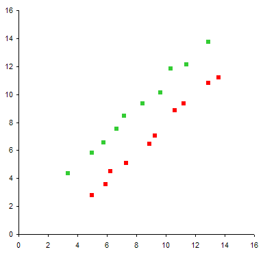
The program was designed to connect corresponding points of two XY series in a chart, with arrows pointing from the point in the first series to its partner in the second. Starting with a chart like this:

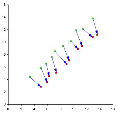
The program produces this effect in Excel 2003 and earlier.

Pretty cool.

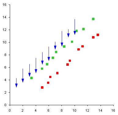
Now run the same procedure on the same chart in Excel 2007, and the result is completely not what you expected. The arrows are all pointing straight downward, and not located near the points they are supposed to connect.

The culprit is the way VBA in Excel 2007 interprets these two lines of code:

    Xnode1 = Xleft + (mySrs1.XValues(Ipts) - Xmin) * Xwidth / (Xmax - Xmin)
    Ynode1 = Ytop + (Ymax - mySrs1.Values(Ipts)) * Yheight / (Ymax - Ymin)
 

These lines provide the X and Y coordinates of the point in the first series (the tail of the arrow), in pixels from the top left of the chart. MySrs1.Values(Ipts) correctly returns the Y value of the point, but MySrs1.XValues(Ipts) returns not the X value of the point, but the index of the point in the series, as text, not as a numeric value.

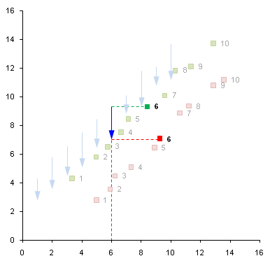
In the chart below, I have highlighted the sixth point in each series and the sixth arrow. We can see that the arrow points from the Y value of point 6 in the first series down to the Y value of point 6 in the second series, while the X value of both endpoints of the arrow is 6.

I can think of another way to create the desired arrows in Excel 2007, and when I have a chance I will write them up.

Stay tuned.

Update 3 June 2009

I discovered that if a chart only has one series, the lines of code above will return the correct X value, though it is still typed as a String.

Update 4 June 2009

On the suggestion of Andy Pope, I downloaded and installed SP2 (I had been using Excel 2007 SP1). As Andy indicates, the code from my earlier article runs fine. The proper X values are extracted from the series data, and they are even typed as doubles.

SP2 fixes the problem. Good job with the update, and sorry to have reported a problem that was already fixed.

I did find another bug, however. I wrote a little routine to spit out chart data into the worksheet, and I used

 With ActiveChart.Parent.TopLeftCell.Offset(, 9)
 

to locate the output of the routine. This works fine in Excel 2003. Excel 2007 SP2 chokes on the Offset method of the Range object, and the line above is highlighted in the debugger.

This works in 2003

 Dim rTopLeft As Range
 Set rTopLeft = ActiveChart.Parent.TopLeftCell
 With rTopLeft.Offset(, 9)
 

but the last line of the above still chokes on Offset. What finally works in 2007 is

With Range(ActiveChart.Parent.TopLeftCell.Address).Offset(, 9)
 

A little work in the Immediate Window shows that it’s TopLeftCell that has the problem.