This is the fourth of a five part series.
Quartiles for Box Plots
This topic is covered in the companion page Quartiles for Box Plots.
Hinge Techniques for Determining Quartiles
This topic is covered in the companion page Hinges.
Interpolation Methods of Determining Quartiles
This topic is covered in the companion page Quartiles.
Comparison of Values from All Hinge and Quartile Methods
Effect of N
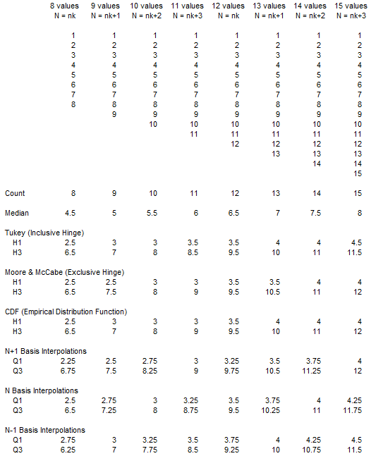
First and third quartiles (or first and second hinges) for N=8 through 15 are tabulated below for all of the quartile determination methods described in the previous sections.
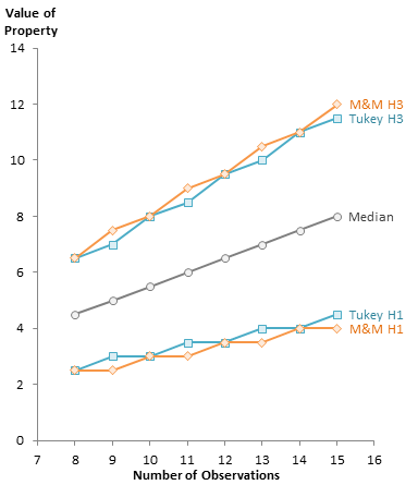
Here the hinges for the Tukey (inclusionary) and the Moore and McCabe (exclusionary) methods are plotted. We see that for even N, the methods result in the same hinges, while for odd N, Tukey is closer to the median, and M&M is further from the median.
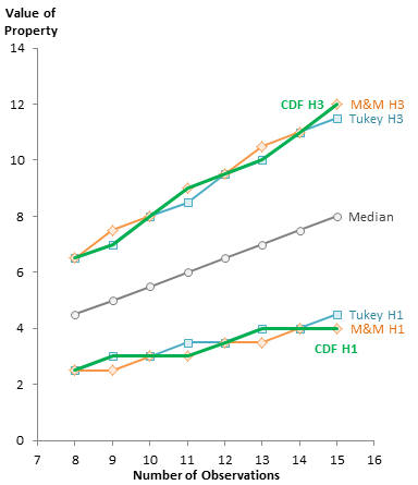
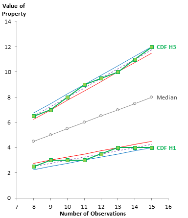
Here the CDF is overlaid on the previous plot of Tukey and M&M. For even N, all techniques agree, while for odd N, the CDF sticks with the method that yields a whole number index.
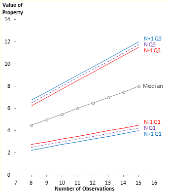
This chart plots the quartile indices for the N+1, N, and N-1 Basis approaches. The N-1 quartiles are closer to the median, the N+1 quartiles are further, and the N are in between. This is the pattern we noticed in the number lines in the previous section.
It becomes interesting when we overlay the various hinge techniques on the N+1/N/N-1 plot. We see that the Tukey hinges is bounded by the N-1 and N quartiles.

The M&M quartiles are bounded by the N and N+1 quartiles.
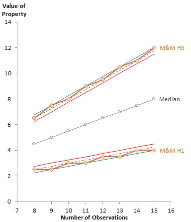
And the CDF hinges are bounded by N+1 and N-1.
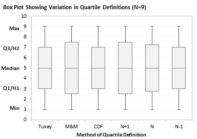
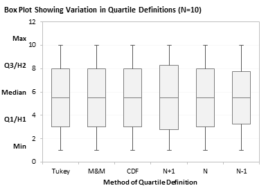
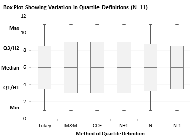
Finally, since these quartiles are intended for use in box plots, here are box plots comparing the six techniques, one box plot each for N=8, 9, 10, and 11.

Doubling the Data Set
Before making any recommendations, let’s see how the techniques compare when we double a data set. For example, if we have a data set of {1,2,3,4,5} and another data set with the same values, but two of each, {1,1,2,2,3,3,4,4,5,5}, we would expect to find the same quartiles. Here is what all the techniques predict.

Forget staring at a table of numbers, the predictions are plotted in the following charts. Any pairs that are not vertically aligned have different quartiles for the data set and its double. These unmatched cases are drawn in orange in the charts below and also in the table above.

Of all the techniques evaluated, only CDF yields the same quartiles for all cases of a data set and its double.
Techniques Used by Software Packages
The following chart rehashes the difference between the N+1 and N-1 techniques for interpolating quartiles. Microsoft Excel’s legacy QUARTILE function uses the N-1 approach, while Minitab, JMP, and other packages use the N+1 approach. Microsoft added two functions to Excel 2010: QUARTILE.INC, which is based on N-1 and is therefore identical to QUARTILE, and QUARTILE.EXC, which is based on N+1. SAS also offers an N+1 option (see below).
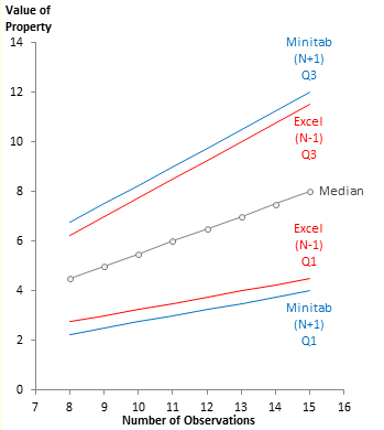
The quartiles for the N-1 technique are closer to the median, so the interquartile range (IQR) is smaller, and the limit for identifying outliers, 1.5IQR above Q3 and below Q1, are also closer to the median.
This means that there are likely to be more outliers identified by Excel than by Minitab. This difference in behavior was a mystery to me a decade ago when my employer provided us with Minitab in addition to Excel, but now it’s very clear. (Many more things were a mystery to the brilliant minds I was stuck working with, but that’s a story for another day, when we’re killing time and beers in the pub.)
The next chart shows the two SAS quartile options. The default is CDF (SAS option PCTLDEF = 5), which as we have seen yields identical quartiles for a data set and the same data set with two of each value. SAS also offers the N+1 option (PCTLDEF = 4), which is used by Minitab, JMP, and Excel’s QUARTILE.EXC. SAS also offers three more options (PCTLDEF 1, 2, and 3), which often produce asymmetric median and quartile definitions, because they round to the larger or closer of two values instead of averaging.
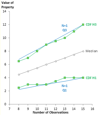
The two sets of results are slightly different, and the CDF quartiles tend to be closer to the median than the N+1 quartiles. As with Excel’s N-1 results, the CDF will have smaller IQR than N+1, leading to identification of more borderline outliers.
Recommendations
So after all this noise, which quartile definition should you use?
The CDF approach is considered by Langford (Quartiles in Elementary Statistics) to be the all-around “best” approach. It is also the default for the powerful software package SAS, though it doesn’t seem to be used in other packages. This may then be the option of choice.
However, an important consideration is consistency. If others you work with are using Minitab or JMP, you should use the N+1 option for compatibility.
Quartiles in the Peltier Tech Chart Utility
This topic is covered in the companion page Quartiles in the Peltier Tech Chart Utility.


DaleW says
Jon,
Great visual presentation and discussion of quartiles! Guess that I will have to fire up my spare PC with Excel 2010 to see what your beta charting utility does with them.
A quartile method that you’ve left out is the recommended “R-8 method” from the 1996 statistical paper by Hyndman and Fan on calculating quantiles of any type. It uses (N+1/3) weighted interpolation to give approximately median-unbiased results. (My favorite statistical add-in for Excel also uses it.)
Jon Peltier says
Dale –
Oh great, you mean I missed a relevant technique? So that’s the (k-1/3)/(N+1/3) one in the paper? I remember using something like (k-1/4)/(N+3/8) years ago when plotting Weibull distributions.
I need to do some other work, then maybe I’ll get back to this.
DaleW says
Jon,
Yes, for when you have more free time again, R-8 is the depth h=(N+1/3)p+1/3 quantile method where p=k/4 for quartiles k={1,2,3 }. This gives nearly unbiased estimates of the median for population order statistics (including quartiles), regardless of distribution. The Analyse-it website gives a nice explanation of why they only use them for box plots in their Excel statistical add-in. You can plot Filliben’s estimate of the median order statistic for a 1st or 3rd quartile vs. N if you want to see how good the N+1/3 Basis is. If you don’t trust Filliben’s 1975 estimate, Monte Carlo simulations of quartiles in Excel (with enormously more computing power than Filliben is likely to have had!) for a few known population distributions and values of N should be quite convincing.
You were probably using the R-9 method where h=(N+1/4)p+3/8 which gives nearly unbiased estimates of the mean for population order statistics when the distribution is normal. This basis can also be useful, now that you mention it, although for box plots it could be risky to assume a normal distribution.
If we demand symmetry from our quantiles (or for quartiles, just that the k=2 median of N numbers be = Np+1/2), then once we select the N-related basis, the intercept constant for h is also determined. If we know h, and h has been limited to the obvious range of 1 to N (a simple and easy correction for our fenceposts regardless of basis) to avoid extrapolation, then our very general quantile or quartile interpolation rule would be simply =SMALL(X,h) — if only SMALL could do linear interpolation for non-integers! Fortunately, you teach how to do linear interpolation between two nearest neighbors in your blog. You won’t be able to use your Choose() one of 4 formulas for interpolated quartiles when the basis is no longer an integer, so the R-8 and R-9 methods would complicate your utility in that sense.
The CDF is a special case of N-based quartiles with fair rounding (0.5 causes us to split the difference), and the inclusive Tukey hinges are a N-based biased rounding (historically significant and logical for quick box plots because both the median and extreme value are already in our 5 number summary), while the exclusive M&M ~hinges are a biased N-based rounding of dubious value in box plots (IMO).
I hope that makes sense . . .