VBA

In recent months I have encountered a particularly troublesome error. It occurs in Excel 2003 and 2007 (and perhaps in earlier versions, but I don’t recall any such cases). The error is heralded by an unusually unhelpful error message, even my Microsoft’s standards: Microsoft Visual Basic – System Error &H80004005 (-2147467259). Unspecified error.

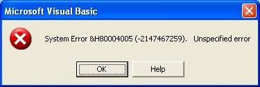
Pardon my French, but WTF?

To rub salt into the wound, this is followed up with an Out of Memory error:

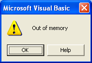
Sometimes these occur once, sometimes twice, when Excel is started, when a workbook with code is opened, or when an add-in is opened.

Association with RefEdit Controls

Closer examination sheds some light on the problem. It seems to be related to our old friend, the RefEdit control. If a workbook or add-in has a UserForm with a RefEdit, this error may occur. When the error occurs, it may be impossible to view the UserForm in the VB Editor, or if the UserForm can be viewed, any RefEdits have been stripped off the form. UserForms without RefEdit controls can be viewed with no problems.

On a computer that experiences the problem, the RefEdit library (refedit.dll) is not available in the references under the VB Editor’s Tools menu,and sometimes it turns up as a MISSING reference in this list. The RefEdit library is also not found in the list of Additional Controls which can be added to the VBE’s Controls Toolbox. If the RefEdit control had been present on the Controls Toolbox, its place may be taken by a gray square with a tooltip of “Unknown”.

Interestingly enough, the RefEdit library is present on the machine, in the Microsoft Office program directory. But the library is apparently not accessible.

There have been some recent changes in the RefEdit control, I believe on more than one occasion, but I have never documented the changes. There are no outwardly visible differences in the control, but the file size has changed, the file created or modified date has changed, and the file version has changed.

History

This famous Unspecified Error, its hex code 80004005 burned into many a programmer’s retinas, has been around for a long time, in Visual Basic 6 and probably earlier. It has been blamed on many factors, many of which seem like wild guesses, and most of which are irrelevant to our situation here. There are a lot of instances in which this error occurred in projects which dealt with retrieval of data from data controls or databases (Access, Oracle, SQL Server, and others). This error has also been associated with ODBC, ADO, IMAP, ASP and IIS, and DLLs from Microsoft (INET and HTML controls) and third parties. I suspect that this is a catch-all error message when there is an internal error in VB, when there is no specific information but the error is somehow associated with various controls or libraries.

At least one Microsoft Knowledge Base article discusses this error in the context of Excel. OFF2000: “System Error &H80004005 (-2147467259)” Running Macro with UserForm attributes the error to opening a file with a userform that contains a Microsoft DirectAnimation Sprite control (daxctle.ocx), whatever that is. Apparently that was the Office 2000 version of the problem, and in Office 2003/2007 it’s kicked off by a RefEdit control.

Google finds innumerable links to this error in web sites and newsgroups, related to Visual Basic, Office, and recently, Excel. I have spent dozens of hours poring through search results looking unsuccessfully for relief.

What makes this problem so much harder to document and troubleshoot is that it does not occur on all computers which have had nominally the same upgrades. One user will be hobbled by this error, while a user in the adjoining cubical will show no signs of it. I have had substantially identical VMs on the same computer, some with the problem, some immune.

Remedies

This problem has surfaced among users of my charting utilities, but usually I’ve been able to fix it. Also, one of my clients has a large Excel add-in package which has experienced this error. So far I think we’ve successfully treated all infections. (And no, I’m not the Excel Doctor.)

I have tried a wide range of remedies. A few involve chicken’s blood at full moon, but most involve various Windows and Office activities. Some remedies work some of the time, but what works on one computer may not work on another.

Because this problem was sporadic when I first encountered it, I didn’t document the exact steps taken to diagnose and remedy the issue. I’ve generally followed a brute force approach until recently.

In mild cases, deleting all files in the user’s temp directory and in the C:\Documents and Settings\User Name\Application Data\Microsoft\Forms directory will clear up the problem. This is all that my main machine needed, but generally it’s like trying to boil the ocean.

Reregistering the refedit.dll does not seem to help. I have tried replacing an older version of this library with a newer version from another computer, but I don’t recall this ever having helped.

Lately it seems that almost all cases in Excel 2003 are fixed using the Help menu’s Detect and Repair command, so this is my first step in treating the malady. Excel 2007 has a similar command deep under the Office Orb (Excel Options > Resources > Run Microsoft Office Diagnostics > Diagnose). I’ve used this command, but it has never given me the same warm fuzzy feeling of a Detect and Repair operation. However, just today an end user ran the diagnostics, and the problem was cleared up.

There are a couple preventative measures which seem to make add-ins resistant to the unspecified error. Open the add-in in Excel 2000, uncheck the reference to the RefEdit library, compile the code (ignoring compile errors related to new Excel 2002-2003-2007 syntax), and save and close the add-in. The compile step may not be necessary. I’ve also removed RefEdit controls and replaced them in 2000, but this seems to be unnecessary (as well as tedious).

I’ve seen two or three cases in which these last few steps did not seem to work. But in at least one of these cases, I’m not sure the end user followed instructions and actually ran the Detect and Repair or Diagnostic command.

Update 23 June 2009

Bob Flanagan has shared a link to his detailed protocols for fixing this and other problems with Office installations at What to do if Excel add-ins do not run. Thanks, Bob.

Other Experiences

Have you encountered this problem? Have you documented it? Have you successfully treated it?

If so, I want to hear about it. Please leave a comment with as many details as you can muster.

In some of the analyses I do, I’ll have a range of data and some charts based on this range. As the analysis unfolds, more columns may be added to the data range, and these have to be added to the chart. Until last week, I would add a series by copying the series formula of an existing series, selecting the plot area, pasting the formula into the formula bar, editing the formula, and pressing Enter. Adding series has been the most tedious part of the analysis, and finally I decided to speed it up.

I wrote some code to create a new series based on the range next to the last series in the chart. The code copies the series formula from the last series, then edits the formula to reference the next column for the name and Y value parameters of the formula. Finally a new series is created, and the edited formula is assigned to this series.

Wonderful! One click to add each new series. Well, a few clicks, but it’s still much faster than the old way.

Then I embellished the routine, added some checks (is a chart selected, is the series formula well-formed, are the ranges readily manipulated, etc.), generalized it to series by rows as well as by columns, and ran a few tests. Worked like a charm.

Here’s a sample chart which initially uses the first three data columns as the Y values for its three series. (With the plot area or chart area selected, the source data range for the chart is highlighted.)

Run the macro: press Alt+F8, select the macro from the list, and click Run.

Here’s the result, which adds the fourth column as the chart’s fourth series.

Naturally, this can be changed using the Source Data dialog, or by dragging the colored outlines that indicate the source data. However, if the existing source data is in a pivot table, the chart would be converted to a pivot chart. Also, if the data is on another worksheet (or multiple worksheets), or if it is discontiguous or even more complicated, this is likely to produce unexpected results, or fail completely.

This procedure only requires that the last series have a series formula that it can parse. The added series is related only to the last series in the chart, using the next row or column in the worksheet.

Here is a chart that initially uses the first three rows of the data range for its three series.

After the macro is run, the chart has four series, using the first four rows of the data range.

Here’s the VBA procedure. If you’re not sure how to implement it, refer to my introductory VBA tutorial, How To: Use Someone Else’s Macro

Sub AddSeriesToEnd()
  '' Add series to active chart
  '' Use same X values
  '' Use Name and Y values one column to right of last existing series
  Dim sFmla As String
  Dim iParen As Long
  Dim sFmlaArgs As String
  Dim vFmlaArgs As Variant
  Dim sMsg As String
  Dim iOffset As Long
  Dim jOffset As Long
  Dim rValues As Range
  Dim rName As Range

  If ActiveChart Is Nothing Then
    sMsg = "Series Formula too complicated to parse"
    GoTo CantHandle
  End If

  With ActiveChart
    sFmla = .SeriesCollection(.SeriesCollection.count).Formula
    iParen = InStr(sFmla, "(")
    sFmlaArgs = Mid$(sFmla, iParen + 1)
    sFmlaArgs = Left$(sFmlaArgs, Len(sFmlaArgs) - 1)
    vFmlaArgs = Split(sFmlaArgs, ",")

    If UBound(vFmlaArgs) + 1 - LBound(vFmlaArgs) <> 4 Then
      sMsg = "Series Formula too complicated to parse"
      GoTo CantHandle
    End If

    On Error Resume Next
    Set rValues = Range(vFmlaArgs(2))
    Set rName = Range(vFmlaArgs(0))
    On Error GoTo 0

    If rValues Is Nothing Then
      sMsg = "Last series values are not in a range"
      GoTo CantHandle
    End If

    If rValues.Rows.count > 1 And rValues.Columns.count = 1 Then
      ' series in columns
      jOffset = 1
    ElseIf rValues.Rows.count = 1 And rValues.Columns.count > 1 Then
      ' series in rows
      iOffset = 1
    Else
      ' one cell or multiple rows and columns
      sMsg = "Series values range cannot be parsed"
      GoTo CantHandle
    End If

    vFmlaArgs(3) = vFmlaArgs(3) + 1
    If Not rName Is Nothing Then
      vFmlaArgs(0) = rName.Offset(iOffset, jOffset).Address(True, True, xlA1, True)
    Else
      vFmlaArgs(0) = "New Series " & vFmlaArgs(3)
    End If
    vFmlaArgs(2) = rValues.Offset(iOffset, jOffset).Address(True, True, xlA1, True)

    sFmlaArgs = Join(vFmlaArgs, ",")
    sFmla = Left$(sFmla, iParen) & sFmlaArgs & ")"
    With .SeriesCollection.NewSeries
      .Formula = sFmla
    End With
  End With

ExitSub:
  Exit Sub

CantHandle:
  MsgBox sMsg, vbCritical + vbOKOnly
  GoTo ExitSub
End Sub