Dynamic ranges (or “Names”) are commonly used to identify a range of the appropriate length, so that a chart will plot the right number of points. For example, you may want to plot year to date sales, without blanks for the months which are still in the future. The dynamic range uses COUNT or similar function to determine how many cells to include. As you add data, the range expands, and the chart automatically adjusts, so it plots all the months to date, but no months beyond that.
You can also use dynamic ranges if you don’t know what column your data is in. You can use MATCH and similar functions to determine which column has a particular header, and selectively plot the data in that column.
I was once given the following task:
We have two systems that produce similar data and need to chart both in a similar manner. However, the exact columns are not the same in each system’s output files and may even move from time to time. I need to do the following:
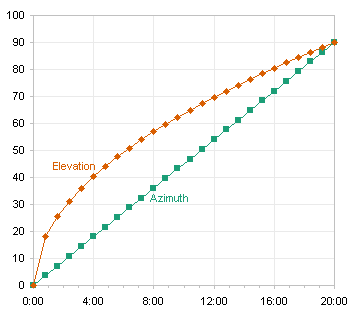
Find the columns containing “Elapsed Time”, “Azimuth”, “Elevation” and chart them with an XY chart with lines connecting the points. The column “Elapsed Time” must the the X axis, while “Azimuth” and “Elevation” are antenna pointing angles that must be plotted on the Y axis.
The following is a sample of the data, with irrelevant columns blanked for this exercise.
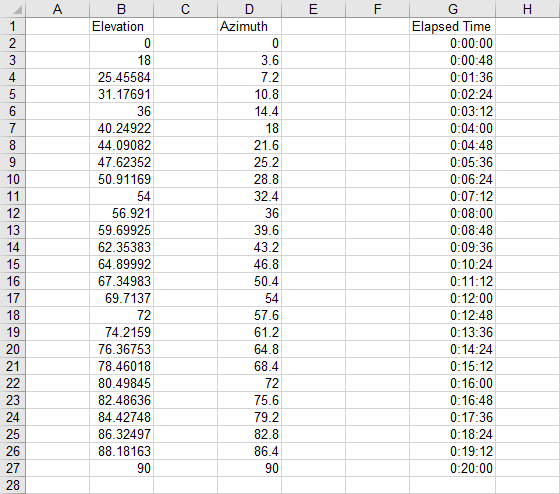
This can be done with dynamic ranges. Assuming the labels are in row 1 of Sheet1, here are some defined names that construct the X and Y value ranges for your chart. Press CTRL+F3 to open the Defined Name dialog, and define these names:
Name: Sheet1!ET
Refers To: =MATCH(“Elapsed Time”,$1:$1,0)
Name: Sheet1!AZ
Refers To: =MATCH(“Azimuth”,$1:$1,0)
Name: Sheet1!EL
Refers To: =MATCH(“Elevation”,$1:$1,0)
(ET, AZ, and EL are the column numbers where these labels are found.)
Name: Sheet1!Xrows
Refers To: =MATCH(1E+307,INDEX($1:$65536,1,ET):INDEX($1:$65536,65536,ET),1)
(This is the number of rows used in the Elapsed Time column)
Name: Sheet1!TheX
Refers To: =(INDEX(Sheet1!$1:$65536,2,ET):INDEX(Sheet1!$1:$65536,Xrows,ET))
Name: Sheet1!TheAZ
Refers To: =(INDEX(Sheet1!$1:$65536,2,AZ):INDEX(Sheet1!$1:$65536,Xrows,AZ))
Name: Sheet1!TheEL
Refers To: =(INDEX(Sheet1!$1:$65536,2,EL):INDEX(Sheet1!$1:$65536,Xrows,EL))
(These are the data ranges under the labels.)
Let’s go to the VB Editor’s Immediate Window to see what we’ve got:
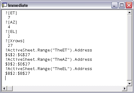
Now use the chart wizard to create a chart. In step 2, click on the Series tab, Select or Add the first series, name it “AZ”, and enter =Sheet1!theX in the X Values box and =Sheet1!theAZ in the Y Values box. Add the second series, again enter =Sheet1!theX in the X Values box, and enter =Sheet1!theEL in the Y Values box. No matter which column has the particular labels (and the left to right alignment doesn’t matter), the dynamic ranges will find the appropriate data for the chart.
