Apply an AutoFilter to an Excel Pivot Table
Excel Pivot Tables are a very powerful feature, and the AutoFilter is also very useful. The row fields of the Pivot Table can be manipulated like an AutoFilter, but the data fields cannot be sorted or filtered. And if you try to apply an AutoFilter to a pivot table, you find the menu command disabled.
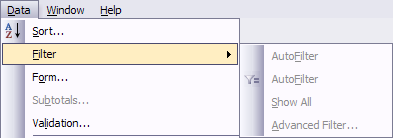
But I learned a trick this week at the Excel Dashboard and Visualization Bootcamp. If you select a cell which borders on the pivot table, but is not part of the pivot table,…

…the AutoFilter menu items are now enabled.

Select AutoFilter, and the Pivot Table has been AutoFilter enabled.

These conferences are great.
AutoFilter by Selection
Access has a feature that lets you quickly apply a filter based on the selected item. Wouldn’t it be great to have this in Excel?
Well, this feature exists, and it’s built in. But it’s not present on the default menus or ribbons. You have to dig it out and install it yourself.
Excel 2003 and earlier
On Excel’s Tools menu, select Customize, click on the Commands tab, select the Data item in the Caegories list, click on the AutoFilter item, and drag it to a convenient place on a toolbar or menu.
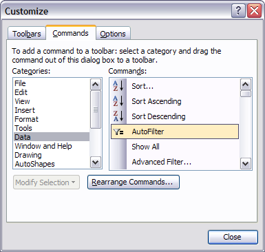
I’ve put this just under the “regular” AutoFilter item on my Data menu/Filter submenu.

Excel 2007
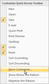
Click on the down arrow to the right of the Quick Access Toolbar, and select More Commands from the popup menu.
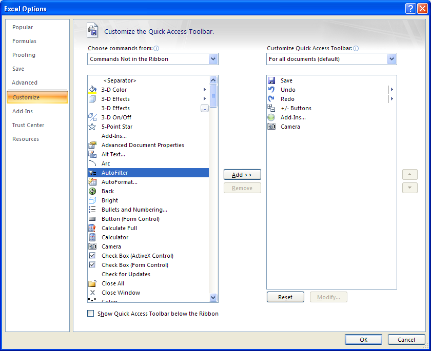
In the oversized dialog that appears, select Commands not in the Ribbon from the right hand dropdown, select AutoFilter, click Add, and press OK.
The AutoFilter icon appears on the QAT.

What the “New” AutoFilter does
This Autofilter command shares a name with the “other” AutoFilter command, but it has a unique icon, and its functionality is enhanced. The command creates an AutoFilter using the range that includes the active cell, then it filters this range based on the active cell.


Debra Dalgleish says
And in Excel 2007 you can right-click on a cell in a autofiltered range, then click Filter>Filter by Selected Cell’s Value (won’t work in your filtered pivot table though)
AdamV says
I like the AutoFilter for Pivot Tables – neat hack.
AutoFilter by selection is useful too, but I use a different way to achieve it in Excel 2007 which I think you will agree may be easier to do*:
whether you have filters turned on already or not, simply right click a cell containing the value you want, then from the context menu go to filter > filter by selected cell’s value (or colour, or font colour, or icon).
If filters were not previously on, they are now turned on for the whole of the contiguous range containing the cell you chose (as usual for filtering and sorting).
When I am training people I describe this as the “show me other things like this one” filter.
It makes it really easy for consumers of data reports to lose the noise – “show me just _my_ sales” or “let me see my division’s performance” or “what else has this customer bought / had fixed / called about in the past”
Once applied, you can also use this to re-apply the same filter quickly if values (…colours, icons) have changed since applying the filter.
Oddly, there does not seem to be a way to clear the filter from this same context menu rather than from the dropdown or from the data ribbon. Add to the 2010 wishlist maybe?
On the subject of clearing filters, if you want to add a button to the QAT (quick access toolbar) to clear all applied filters (but leaving the filters in place), you need to use the button labelled “Clear” from the Data ribbon collection (just right click it > add to QAT). (this clears filters and applied sort orders, but the latter seems irrelevant, it does not re-sort data back into the original order or anything like that, but it does “forget” how it arrived at the current order of your data).
If you customise the QAT and add the button called “Clear filters” from the “Commands not found in the ribbon” list, it does not work. In fact it is disabled…until you have a pivot table selected with filters applied, then this is the right button to use to clear all filters and make sure you are looking at a report of all the underlying data with nothing hidden.
* so my way takes three clicks instead of your two, but they are in a smaller region of the screen and don’t require you to pre-prepare the QAT with a custom button.
Also as an aside, in 2007 the ‘normal’ Filter button and the “AutoFilter like this one” button look the same, both have the equals sign on (unlike the large button on the Data ribbon which is a plain funnel picture). This may be something to do with the fact that the menu choice had no icon in Excel 2003 so they simply picked one from the existing set to use in the new version. Poor choice.
Matt Healy says
Great post. I thought I knew all the wrinkles of Autofilter but you’ve shown me a few more that I did not know.
Autofilter is one of the most powerful and under-appreciated features of Excel. I use it in most of the reports I provide to my clients, and when I deliver the report I ask them to schedule a one-hour session so I can go over the report with them. Usually more than half of that hour is spent showing them how they can use Autofilter to drill-down on parts of the data of interest to them. I put significant effort into laying out my reports so as to maximize the value of Autofilter.
jeff weir says
Hi John. From memory, a problem with using autofilter like this is that if you subsequently use a filter on one of the pivot table row fields you can get some nonsensical results because there’s some conflict between the autofiltered fields and the pivot table row fields. Can’t quite remember the specifics, and the offending file is at work…so I’ll update this with more specifics if I can.
What I did to overcome this is turn whatever info in the pivot table data fields into aggregate totals using a bit of SQL, and then made them all pivot table row fields. This worked a treat.
Lori says
This is a neat trick.
It also allows an easy way to create custom groupings within the table:
– apply the filter eg contains “XYZ”,
– select the visible cells in the customers column (shortcut: Alt + ;)
– group data into “XYZ” and other categories “Non-XYZ”.
Simillarly advanced filter also works if the command is selected with a cell outside the pivot table which can be useful for doing data completeness checks.
Roger Govier says
That’s a neat trick, adding the Autofilter to a Pivot Table.
Thanks for sharing.
derek says
I have had the Autofilter by selection button in my XL97 and 2000 toolbars for so long I had forgotten they were a “trick”. I enthusiastically endorse adding it to your toolbar; it’s something I use every day. The Autofilter Pivot Table trick is neat, I must see what I can do with it at work.
Here’s another Excel trick I use every day that I forgot was a trick. Double-click on a formula and it takes you to the first referenced cell off page, if the first referenced cell is off the page. If the first referenced cell is on the page, it selects all the referenced cells on the page, and you can step through them all using Tab.
This is great for debugging a spreadsheet, but I was shocked to realise most of my colleagues don’t have it! When they double-click on a cell, it opens the cell for editing (I always edit in the formula bar above, never in the cell).
And I couldn’t tell them how I get the drilldown function. Is it simply a matter of turning off “Edit directly in cell” in Tools.. Options.. Edit?
iesmatauw says
wow, just reading the first trick already make my head to think about a few useful changes to my weekly reports.
Jon Peltier says
Derek –
That’s a neat trick, too. Have to try it.
AlexJ says
Found a couple issues with Pivot Table Filtering. It works nicely for a “flat” table as you present, Jon, but unfortunately, if you use Outline groupings on fields with subtotals at top (which is one of my preferences), then you only get the subtotal line under the filter, not the whole group.
Also, if you add a line between outline groups, the autofilter does not pick up the whole table, just the first section.
Luckily, I found for this kind of table that double click on Outline group headers toggles visibility of the detail data. Also, the icons from the [Data] [Group and Outline] menu work on this style of pivot table – I bring those icons out onto a custom toolbar for quick access.
jeff weir says
I stumbled across a neat hack today re filtering pivottables that’s so obvious it has been right under my nose.
As I point out above, a problem with using a filter down the side of a pivottable to filter it can cause some issues if you are also using filters in the pivot fields. And as I also mentioned above, I’ve previously been aggregating up some of my pivot table data fields into aggregate totals using a bit of SQL, so that they could then be dropped in to the pivottable as row fields and filtered.
But today, I tried a different tack, after realising a pivottable can be used as a datasource for another pivot table.
One bonus of this method is that you can effectively add ad-hoc fields to your original (Master) pivottable, that then show up fully intergrated in the new (Slave) pivottable. That is, you can build some ad-hoc formulas that far surpass what a calculated field will allow you to do, or introduce new data altogether (perhaps from a seperate data source, as I was doing today). This can then be dragged and dropped into the new pivot table as row fields or data fields, just like the original data can. So you can happily filter away, as well as sort the Slave pivot table by the new fields (which you can’t do with the autofilter hack above).
For instance, if you want your dates to coincide with a fiscal year that runs from 1 July, but you can’t get at the original data source to add another field, or you want a quick and dirty workaround, then you could put a new column to the left of your original pivottable (rather than the right, where it would get overwritten if the Master Pivot Table has any more row or data fields added to it) and use the formula to return a financial year field, using something like:
=IF(MONTH(B2)>6,YEAR(B2)+1,YEAR(B12)) …assuming this formula is in A2 and copied down, and the pivottable has dates in row B2, and you put ‘financial year’ as a header in A1
Then when you selet the data source for the Slave pivot table, just be sure to include row A through to the last row that has pivot table data, and you’ve solved your problem. Probably best to define a dynamic range for this in case the Master pivot table grows or shrinks.
This might be a convenient way to bring new data into a pivotchart too…if pivot charts are your thing.
What do you think? Worthwhile? Drawbacks?
Jon Peltier says
Jeff –
This is a neat trick, and one that I’ve resorted to when the calculated fields didn’t calculate what I wanted.
You know how to get the original data out of a pivot table, don’t you? Double clicking on any cell in a pivot table inserts a new sheet with the records used to calculate that cell. Double clicking on the grand total cell gives you all records in the original source data.
athinaok says
Thank you very much you saved me from hours of programming!
Jeff Weir says
Here’s a strange wee bug, related to this post. This screenshot of an excel 2007 pivottable shows the options available for a row field.
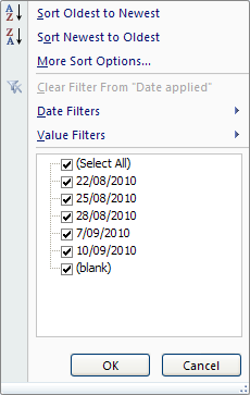
If you then add an autofilter to a pivot table the way mentioned above, then here’s what you see:
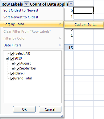
The option that used to read ‘More sort options’ now reads ‘Sort by Color’….although it in fact allows you to click on the ‘Custom Sort’ button and sort by something actually useful.
Tracy says
Thanks so much for the post. It saves a lot of time for me. I am so pleased to have find the post, have been trying to get filter working in VBA for hours.
Tamara says
Thanks for this post, I’ve just upgraded to 2010 and panicked because the autofilter wasn’t there but your post helped me find it :)
BI User says
Thank you for the tip. Great post!
Miv says
Also – just a note for the keyboard warriors out there. The shortcut to toggle advanced filters on and off is [CTRL+SHIFT+L]
Also, the keyboard combination to clear filters is: ALT, A, C
Personally I type considerably faster than I can move a mouse!