Assign Chart Series Names or Categories with VBA

Ask User for a Range

VBA provides a number of ways to interact with users. MsgBox lets you send a message to a user, and get a simple response (yes/no or okay/cancel) in return. InputBox lets you ask a user to input some information. And you can design a whole UserForm as a custom dialog.

We will use an InputBox to get a range from our user. There are two kinds of InputBox: regular InputBox that accepts text input from the user, and Application.InputBox, which lets you require a certain type of information from the user. Since we need a range, we’ll use Application.InputBox. The required syntax is:

Function InputBox(Prompt As String, [Title], [Default], _
    [Left], [Top], [HelpFile], [HelpContextID], [Type])

You supply a Prompt to tell the user what you need, and optionally a Title for the InputBox and a Default value. Left and Top position the InputBox but haven’t worked in recent memory. HelpFile and HelpContextID are used if you have help content for the InputBox. Finally, Type describes the type of data you want; for our purposes, type 8 is used for a range.

Here is a simple VBA procedure that uses Application.InputBox. It uses simple prompt, title, and default arguments, plus the 8 for range, and the in between arguments are left blank. When a range is returned, those cells are filled red.

Sub GetUserRange1()
  Dim UserRange As Range
  Set UserRange = Application.InputBox("Prompt", "Title", "$A$1", , , , , 8)
  UserRange.Interior.Color = vbRed
End Sub

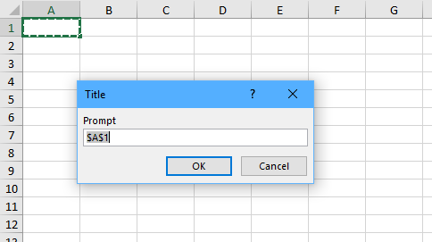
When the code runs, here is how it looks. The default range is highlighted with a dark dashed outline.

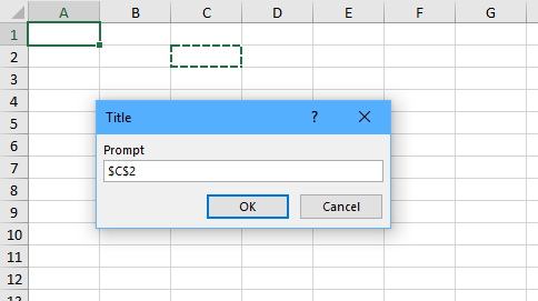
When another range is selected, its address appears in the InputBox, and the new range is highlighted a dark dashed outline.

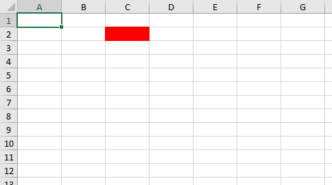
When we then click OK, the selected cell is filled red.

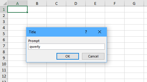
If we try to enter anything that isn’t a range, we get a warning.

If we give up and hit cancel, we get a run time error. The statement calling InputBox is highlighted.

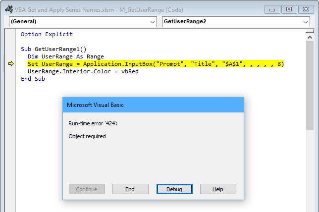
The warning is fine, but we don’t want to saddle our poor user with the run time error, so we will make a minor modification to the code. Actually, two modifications. First, we wrap the call to InputBox in On Error Resume Next and On Error GoTo 0. Then, if the user has canceled, UserRange will not have been assigned, so it is Nothing, and if this is the case, we’ll bail out before trying to format a nonexistent range, which would lead to another error.

Sub GetUserRange2()
  Dim UserRange As Range
  On Error Resume Next
  Set UserRange = Application.InputBox("Prompt", "Title", "$A$1", , , , , 8)
  On Error GoTo 0
  If UserRange Is Nothing Then Exit Sub
  UserRange.Interior.Color = vbRed
End Sub

Execution exits the sub above in two places, either Exit Sub if UserRange Is Nothing or End Sub at the end. If you have a bit of OCD like I do, you’d prefer the code to always exit at one place, so I usually use this structure instead:

Sub GetUserRange2A()
  Dim UserRange As Range
  On Error Resume Next
  Set UserRange = Application.InputBox("Prompt", "Title", "$A$1", , , , , 8)
  On Error GoTo 0
  If Not UserRange Is Nothing Then
    UserRange.Interior.Color = vbRed
  End If
End Sub

Let’s punch up the code with a few text variables, and allow for a smart default range (or you can omit the default to leave out blank if that makes more sense).

Sub GetUserRange3()
  Dim Prompt As String
  Prompt = "Select a Range"
  Dim Title As String
  Title = "Select Range"
  Dim Default As String
  Default = "$A$1"
  If TypeName(Selection) = "Range" Then
    Default = Selection.Address(True, True)
  End If
  Dim UserRange As Range
  On Error Resume Next
  Set UserRange = Application.InputBox(Prompt, Title, Default, , , , , 8)
  On Error GoTo 0
  If Not UserRange Is Nothing Then
    UserRange.Interior.Color = vbRed
  End If
End Sub

So now that we know how to get a range from the user, let’s put it to better use than just formatting a range to have a red background.

Select Range and Assign Series Names

In this example, we’ll ask the user for a range containing series names, and we’ll apply the range to the active chart’s series one by one, until we run out of series in the chart or cells in the selected range.

Since we’re working on the active chart, the user must select a chart before running the code. We’ll use this structure to make sure there is an active chart:

Sub DoSomethingToActiveChart()
   If ActiveChart Is Nothing Then
     MsgBox "Select a chart and try again.", vbExclamation, "No Chart Selected"
   Else
     ' do our thing here
   End If
 End Sub

Often I just bail out if there’s no active chart, but it’s nice to let the user know why nothing happened when they clicked a button.

In the procedure below, we check first for an active chart, then we ask for a range containing series names. Then we make sure the range is a single row or column (not strictly necessary, but otherwise it gets complicated), and step through the series of the chart, using each cell in the range as the title of the series.

Sub SelectRangeWithSeriesNames()
   If ActiveChart Is Nothing Then
     MsgBox "Select a chart and try again.", vbExclamation, "No Chart Selected"
   Else
     Dim Prompt As String
     Prompt = "Select a range that contains series names for the active chart."
     Dim Title As String
     Title = "Select Series Names"
     Dim SeriesNameRange As Range
     On Error Resume Next
     Set SeriesNameRange = Application.InputBox(Prompt, Title, , , , , , 8)
     On Error GoTo 0
     If Not SeriesNameRange Is Nothing Then
       If SeriesNameRange.Rows.Count = 1 Or SeriesNameRange.Columns.Count = 1 Then
         With ActiveChart
           Dim iSrs As Long
           For iSrs = 1 To .SeriesCollection.Count
             If iSrs <= SeriesNameRange.Cells.Count Then
               .SeriesCollection(iSrs).Name = _
                   "=" & SeriesNameRange.Cells(iSrs).Address(, , , True)
             End If
           Next
         End With
       Else
         MsgBox "Select a range with one row or one column", vbExclamation, _
             "Must be One Row or Column"
       End If
     End If
   End If
 End Sub

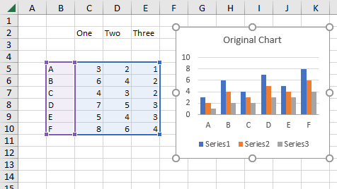
Here is a chart. The highlighted data range shows that the Y values are in C5:E10, and the category labels (X values) in B5:B10, but no series names are highlighted. The series names Series1 etc. in the legend also indicate that no series names have been specified.

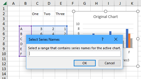
Let’s use the labels in C2:E2 for series names. Run the code: the InputBox is waiting for a range to be selected.

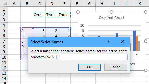
Select a range: it is highlighted with a dark dashed outline.

Click OK and the selected range is now highlighted as the series names, and the chart legend shows these labels as series names.

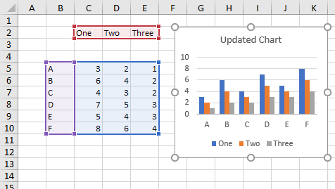
The above procedure can be used to assign series names (legend entries) for a chart that has none, or to replace the existing names (entries) in a chart that already has them.

If there are not enough cells in the selected range, some series do not get new names assigned. If there are more cells than series, the code ignores the excess cells.

Select Range and Assign Categories

In much the same way, we can ask a user for a range containing category labels (X axis values) to assign to a chart.

Sub SelectRangeWithCategoryLabels()
   If ActiveChart Is Nothing Then
     MsgBox "Select a chart and try again.", vbExclamation, "No Chart Selected"
   Else
     Dim Prompt As String
     Prompt = "Select a range that contains category labels for the active chart."
     Dim Title As String
     Title = "Select Category Labels"
     Dim CategoryLabelRange As Range
     On Error Resume Next
     Set CategoryLabelRange = Application.InputBox(Prompt, Title, , , , , , 8)
     On Error GoTo 0
     If Not CategoryLabelRange Is Nothing Then
       If CategoryLabelRange.Rows.Count = 1 Or CategoryLabelRange.Columns.Count = 1 Then
         With ActiveChart
           If CategoryLabelRange.Cells.Count = .SeriesCollection(1).Points.Count Then
             .SeriesCollection(1).XValues = CategoryLabelRange
           Else
             MsgBox "Select a range with the correct number of points.", vbExclamation, _
                 "Wrong Number of Points"
           End If
         End With
       Else
         MsgBox "Select a range with one row or one column", vbExclamation, _
             "Must be One Row or Column"
       End If
     End If
   End If
 End Sub

The above procedure can be used to assign category labels (X axis values) for a chart that has none, or to replace the existing labels in a chart that already has them.

The selected range must have one row and multiple columns or one column and multiple rows. (In some cases, a chart can have category labels that use multiple rows/columns, but that is a lot more complicated than needed for this example.) If this condition is not met, the code tells the user to try again.

Here is a chart. The highlighted data range shows that the Y values are in D3:F8, and the series names in D2:F2, but no categories are highlighted. The category labels 1, 2, 3, etc. along the X axis also indicate that no categories have been specified.

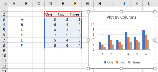
Let’s use the labels in B3:B8 for categories. Run the code: the InputBox is waiting for a range to be selected.

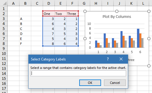
Select a range: it is highlighted with a dark dashed outline.

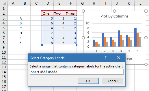
Click OK and the selected range is now highlighted as the category range, and the horizontal axis displays these labels as categories.

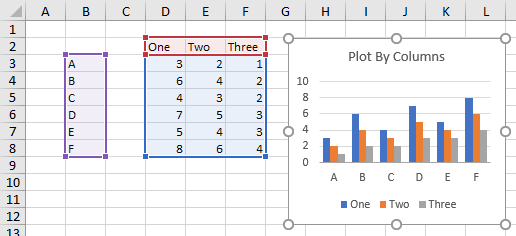
The above procedure can be used to assign categories (X values) for a chart that has none, or to replace the existing categories in a chart that already has them.

If the selected range has the wrong number of cells for the points in a series, the procedure tells the user to select a range with the right number of labels.

Find Range and Assign Series Names

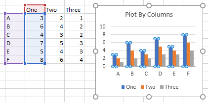
If we construct a chart from an ideally-shaped range, there is a predictable alignment of X values, Y values, and series names in the worksheet. In this chart, the series data is in columns. The Y values for a series are in a vertical range, and the series name is in the cell directly above these Y values. The category labels (X values) are in the column to the left of the Y values of the first series.

In the next chart, the series data is in rows. The Y values for a series are in a horizontal range, and the series name is in the cell directly to the left these Y values. The X values are in the row above the Y values of the first series.

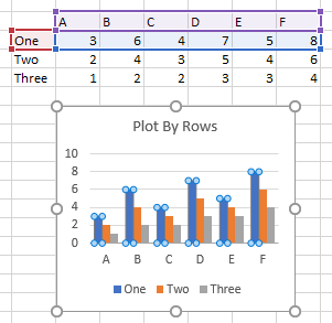
If for some reason the chart was constructed without series names or without category labels, but the missing elements are in the right alignment with respect to the Y values, we can find the cells with the series names or category labels and assign them to the chart.

Find Range and Assign Series Names

The procedure below processes each series in the active chart. First it looks up the SERIES formula, and extracts its arguments into an array. The code finds the address of the Y values, which is in the third argument, and locates the associated range. Then it determines whether the data is by column or by row, identifies the cell with the series name, and uses this cell’s address as the name of the series.

Sub FindAndApplyNamesToSeries()
   If Not ActiveChart Is Nothing Then
     With ActiveChart
       Dim srs As Series
       For Each srs In .SeriesCollection
         ' series formula
         Dim sFmla As String
         sFmla = srs.Formula
         ' just the arguments
         sFmla = Mid$(Left$(sFmla, Len(sFmla) - 1), InStr(sFmla, "(") + 1)
         ' split into an array
         Dim vFmla As Variant
         vFmla = Split(sFmla, ",")
         ' Y values are the 3rd argument
         Dim sYVals As String
         sYVals = vFmla(LBound(vFmla) + 2)
         ' the Y value range
         Dim rYVals As Range
         Set rYVals = Range(sYVals)
         ' by row or column?
         If rYVals.Rows.Count > 1 Then
           ' by column, so use cell above column of Y values
           Dim rName As Range
           Set rName = rYVals.Offset(-1).Resize(1)
         ElseIf rYVals.Columns.Count > 1 Then
           ' by row, so use cell to left of Y values
           Set rName = rYVals.Offset(, -1).Resize(, 1)
         Else
           ' one cell only: who knows?
           Set rName = Nothing
         End If
         If Not rName Is Nothing Then
           srs.Name = "=" & rName.Address(, , , True)
         End If
       Next
     End With
   End If
 End Sub

The data range for the chart below is intact, but somehow, the series names were not associated with it.

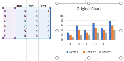
Select the chart and run the procedure, and it applies the series names.

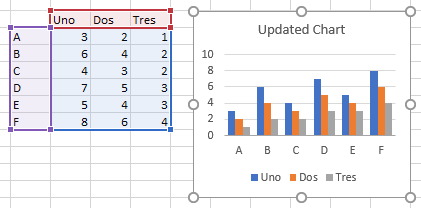
If the series in the chart already had names, this procedure overwrites those names with the names it finds in the worksheet.

Find Range and Assign Categories

The procedure below processes the first series in the active chart. First it looks up the SERIES formula, and extracts its arguments into an array. The code finds the address of the Y values, which is in the third argument, and locates the associated range. Then it determines whether the data is by column or by row, identifies the parallel range with the categories (X values), and uses this range as the categories for the first series, and therefore, for the chart.

Sub FindAndApplyCategoriesToChart()
   If Not ActiveChart Is Nothing Then
     With ActiveChart
       Dim srs As Series
       Set srs = .SeriesCollection(1)
       ' series formula
       Dim sFmla As String
       sFmla = srs.Formula
       ' just the arguments
       sFmla = Mid$(Left$(sFmla, Len(sFmla) - 1), InStr(sFmla, "(") + 1)
       ' split into an array
       Dim vFmla As Variant
       vFmla = Split(sFmla, ",")
       ' Y values are the 3rd argument
       Dim sYVals As String
       sYVals = vFmla(LBound(vFmla) + 2)
       ' the Y value range
       Dim rYVals As Range
       Set rYVals = Range(sYVals)
       ' by row or column?
       If rYVals.Rows.Count > 1 Then
         ' by column, so use column to left of Y values
         Dim rXVals As Range
         Set rXVals = rYVals.Offset(, -1)
       ElseIf rYVals.Columns.Count > 1 Then
         ' by row, so use row above Y values
         Set rXVals = rYVals.Offset(-1)
       Else
         ' one cell only: who knows?
         Set rXVals = Nothing
       End If
       If Not rXVals Is Nothing Then
         srs.XValues = rXVals
       End If
     End With
   End If
 End Sub

The data range for the chart below is intact, but somehow, the categories were not attached to it.

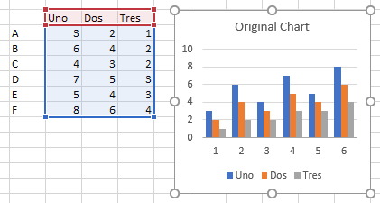
Select the chart and run the procedure, and it applies the categories to the chart.

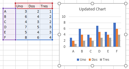
If the series in the chart already had categories, this procedure overwrites those categories with the new labels it finds in the worksheet.

Select Chart Source Data Range

For completeness, here is the routine that lets the user select the chart source data for the active chart.

Sub SelectChartSourceDataRange()
   If ActiveChart Is Nothing Then
     MsgBox "Select a chart and try again.", vbExclamation, "No Chart Selected"
   Else
     Dim Prompt As String
     Prompt = "Select a range that contains source data for the active chart."
     Dim Title As String
     Title = "Select Chart Source Data Range"
     Dim ChartSourceData As Range
     On Error Resume Next
     Set ChartSourceData = Application.InputBox(Prompt, Title, , , , , , 8)
     On Error GoTo 0
     If Not ChartSourceData Is Nothing Then
       ' if a range was selected
       If ChartSourceData.Rows.Count >= ChartSourceData.Columns.Count Then
         Dim DataOrientation As XlRowCol
         DataOrientation = xlColumns
       Else
         DataOrientation = xlRows
       End If
       ActiveChart.SetSourceData ChartSourceData, DataOrientation
     End If
   End If
 End Sub

Jon’s Toolbox

If you follow this blog closely, you may have heard of Jon’s Toolbox, a new Excel add-in that I released recently. I’ve already made a few changes to this utility, thanks to suggestions from readers like you.

Jon’s Toolbox already had a feature that made it easy to select a new source data range for a chart. While finishing up this article, I realized that these features should be included in the software.

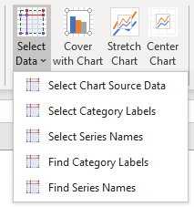
The features have only been added to the DEV version of the software on my computer, but in a week or so I will release a new build that includes these new functions. If you already have Jon’s Toolbox, subscribe to my newsletter to hear when the new build is live. If you don’t have Jon’s Toolbox, you can get it at the bottom of my article Jon’s Toolbox – A New Utility from Peltier Tech.