The report you submitted at the end of last year was well received. Your brilliant analysis was backed up by informative charts. Your boss, his boss, and the shareholders were all very impressed.
Now you have to update the chart to show year to date information, but you don’t want to generate all new charts. You also would rather not go through the hassle of copying data and pasting it into each chart, or worse, navigate the source data dialog umpteen times.
Here’s your old pal Jon with a time saving VBA routine to update your charts painlessly.
Last Year’s Report
In your acclaimed report, you compared 2008 and 2009 monthly sales. Very nice, the generally increasing trend seen in 2008 continued in 2009. Must be a fine product.
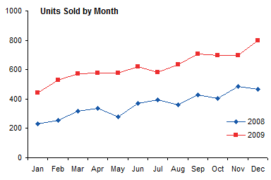
The data for this chart is in a simple table, shown below with the source data highlighted by selecting the chart.
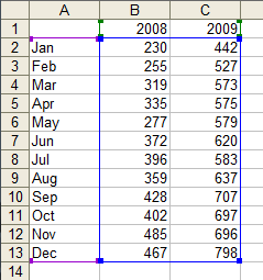
The Interim Report
In the intervening months, sales data for 2010 has been generated, in the next column of the table. Now we have to add this data to the chart.
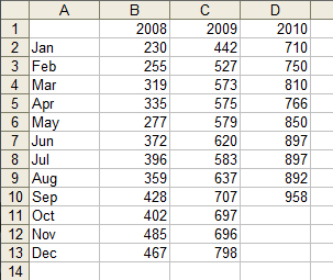
All that is needed is to select the chart and run the VBA procedure below. The code starts with the series formula of the last series in the chart:
=SERIES(Report!$C$1,Report!$A$2:$A$13,Report!$C$2:$C$13,2)which contains the series source data as follows:
=SERIES(Name,X_Values,Y_Values,Plot_Order)The code extracts the Y_Values argument, then depending on the orientation of this data, determines the next column or row of data to use for the Y values of a new series.
If the name of the existing last series was taken from the worksheet, then the corresponding cell in the next column or row will provide the name for the new series; otherwise, the generic name “Series N” will be used. The new series will use the same X values as the existing last series.
The code adds a new series with the old X values, the new Y values and series name, and a plot order one higher than the last:
=SERIES(Report!$D$1,Report!$A$2:$A$13,Report!$D$2:$D$13,3)Here is the resulting chart:
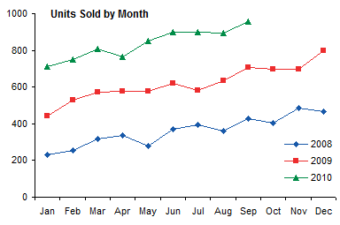
Awesome, monthly sales have followed the upward trend. When we select the chart, we can easily see that the source data now includes the range for the new series.
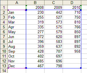
The code is listed below. It’s not too complicated, and includes a little bit of error handling in case you forgot to select a chart before running it, or in case the series formula of the last series cannot be parsed into something useful.
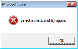
It’s common courtesy to give the user a meaningful explanation of why your code crapped out (or why they broke it):
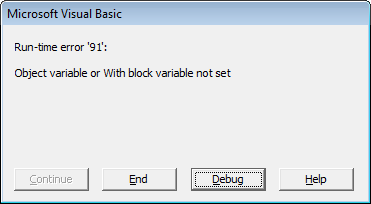
The alternative is ugly.
Sub AddSeriesToEnd()
  ' Add series to active chart
  ' Use same X values
  ' Use Name and Y values one column to right of last existing series
  Dim sFmla As String
  Dim iParen As Long
  Dim sFmlaArgs As String
  Dim vFmlaArgs As Variant
  Dim sMsg As String
  Dim iOffset As Long
  Dim jOffset As Long
  Dim rValues As Range
  Dim rName As Range

  If ActiveChart Is Nothing Then
    sMsg = "Select a chart, and try again."
    GoTo CantHandle
  End If

  With ActiveChart
    sFmla = .SeriesCollection(.SeriesCollection.Count).Formula
    iParen = InStr(sFmla, "(")
    sFmlaArgs = Mid$(sFmla, iParen + 1)
    sFmlaArgs = Left$(sFmlaArgs, Len(sFmlaArgs) - 1)
    vFmlaArgs = Split(sFmlaArgs, ",")

    If UBound(vFmlaArgs) + 1 - LBound(vFmlaArgs) <> 4 Then
      sMsg = "Series Formula too complicated to parse"
      GoTo CantHandle
    End If

    On Error Resume Next
    Set rValues = Range(vFmlaArgs(2))
    Set rName = Range(vFmlaArgs(0))
    On Error GoTo 0

    If rValues Is Nothing Then
      sMsg = "Last series values are not in a range"
      GoTo CantHandle
    End If

    If rValues.Rows.Count > 1 And rValues.Columns.Count = 1 Then
      ' series in columns, so offset 1 column
      jOffset = 1
    ElseIf rValues.Rows.Count > 1 And rValues.Columns.Count = 1 Then
      ' series in rows, so offset 1 row
      iOffset = 1
    Else
      ' one cell or multiple rows and columns
      sMsg = "Series values range cannot be parsed"
      GoTo CantHandle
    End If

    vFmlaArgs(3) = vFmlaArgs(3) + 1
    If Not rName Is Nothing Then
      vFmlaArgs(0) = rName.Offset(iOffset, jOffset).Address(True, True, xlA1, True)
    Else
      vFmlaArgs(0) = "New Series " & vFmlaArgs(3)
    End If
    vFmlaArgs(2) = rValues.Offset(iOffset, jOffset).Address(True, True, xlA1, True)

    sFmlaArgs = Join(vFmlaArgs, ",")
    sFmla = Left$(sFmla, iParen) & sFmlaArgs & ")"
    With .SeriesCollection.NewSeries
      .Formula = sFmla
    End With
  End With

ExitSub:
  Exit Sub

CantHandle:
  ' display generated error message
  MsgBox sMsg, vbCritical + vbOKOnly
  GoTo ExitSub
End Sub
If you’re not sure how to make use of this code, please read How To Use Someone Else’s Macro.


Mike says
Hi Jon
Great tutorial this is a great solution to one of the problems I have at work in terms of adding new series to multiple charts at work. I’m just having some difficulty getting the code to work.
If I don’t choose a chart the appropriate warning comes up as per the macro however when I select the chart and run the macros it adds series three but no values? Not sure what I’m doing wrong
Mike
Jon Peltier says
Mike –
I just copied the code from the web page and pasted it into a module, and it worked as expected. What’s your data look like?
Eugene, Ukraine says
Many thanks for your work, Jon!
It helped me a lot!
Mike says
Jon
When I copy the code from the site into the VBA editor it loses its formatting and becomes one continuous line. Is there a way to get it to keep its line format?
Here is the code which I’ve copied from your site and formatted in VB editor when I run the macro it generates error “unable to set the formula property of the series class” a series 3 is generated but without y values:
Sub AddSeriesToEnd()
” Add series to active chart
” Use same X values
” Use Name and Y values one column to right of last existing series
Dim sFmla As String
Dim iParen As Long
Dim sFmlaArgs As String
Dim vFmlaArgs As Variant
Dim sMsg As String
Dim iOffset As Long
Dim jOffset As Long
Dim rValues As Range
Dim rName As Range
If ActiveChart Is Nothing Then
sMsg = “Select a chart, and try again.”
GoTo CantHandle
End If
With ActiveChart
sFmla = .SeriesCollection(.SeriesCollection.Count).Formula
iParen = InStr(sFmla, “(“)
sFmlaArgs = Mid$(sFmla, iParen + 1)
sFmlaArgs = Left$(sFmlaArgs, Len(sFmlaArgs) – 1)
vFmlaArgs = Split(sFmlaArgs, “,”)
If UBound(vFmlaArgs) + 1 – LBound(vFmlaArgs) 4 Then
sMsg = “Series Formula too complicated to parse”
GoTo CantHandle
End If
On Error Resume Next
Set rValues = Range(vFmlaArgs(2))
Set rName = Range(vFmlaArgs(0))
On Error GoTo 0
If rValues Is Nothing Then
sMsg = “Last series values are not in a range”
GoTo CantHandle
End If
If rValues.Rows.Count > 1 And rValues.Columns.Count = 1 Then
‘ series in columns, so offset 1 column
jOffset = 1
ElseIf rValues.Rows.Count > 1 And rValues.Columns.Count = 1 Then
‘ series in rows, so offset 1 row
iOffset = 1
Else
‘ one cell or multiple rows and columns
sMsg = “Series values range cannot be parsed”
GoTo CantHandle
End If
vFmlaArgs(3) = vFmlaArgs(3) + 1
If Not rName Is Nothing Then
vFmlaArgs(0) = rName.Offset(iOffset, jOffset).Address(True, True, xlA1, True)
Else
vFmlaArgs(0) = “New Series ” & vFmlaArgs(3)
End If
vFmlaArgs(2) = rValues.Offset(iOffset, jOffset).Address(True, True, xlA1, True)
sFmlaArgs = Join(vFmlaArgs, “,”)
sFmla = Left$(sFmla, iParen) & sFmlaArgs & “)”
With .SeriesCollection.NewSeries
.Formula = sFmla
End With
End With
ExitSub:
Exit Sub
CantHandle:
‘ display generated error message
MsgBox sMsg, vbCritical + vbOKOnly
GoTo ExitSub
End Sub
thnx Mike
Jon Peltier says
Mike –
I don’t know what’s up with the code. I got one long string when I copied it too. I ended up copying it from the page source.
Note that in the code, all quotes are straight quotes, not the curly quotes that WordPress insists on using. Quotes at the beginning of a line are single quotes (sometimes two single quotes) to indicate comments. Quotes within a line are double quotes. This line:
If UBound(vFmlaArgs) + 1 – LBound(vFmlaArgs) 4 Then
needs less than and greater than signes before the 4.
I made these adjustments to what you pasted into your comment, and it worked fine.
Pratish says
Jon, thanks for a very useful post – have been cutting and pasting series data into charts and manually formatting it (when it works as expected that is!).. didn’t realise I could do it so easily with VBA
Kalle says
Hi John,
I know this is not connected to this post but I have a question for you. Me and a friend of mine have been trying to come with a good way to do a Nightingale’s Rose in Excel. Is that something you would know how to do? This is an example of what we want to be able to do:
Thanks!
/Kalle
Jon Peltier says
Hi Kalle –
An article on the same site as the picture you cited, Nightingale’s Rose, explains why the polar area plot (or Nightingale’s rose) is attractive, but not too easy to read. The article shows a few alternative approaches to plotting the same data in such a way that it can actually be read.
Kalle says
Hi Jon.
Yes i did read that. And I do agree that it is hard to beat a stacked bar chart. But for our project that would’t work cause it would be to “common”. So do you think one can create a the Nightingale’s Rose in excel?
Thanks allot!
Kalle
Eric says
Jon,
I need to be able to hide or show a series, and the only way that I can think to do this right now is by deleting a series to hide it and adding a series to show it (the data would persist in a spreadsheet – only the line on the chart would be going away or reappearing). Is there something in the object model that I’m missing – a visible property someplace – that would make this so much easier?
Thanks for your help,
Eric
Eric says
Jon,
I just found your entry “Interactive Multiple Line Chart” which, I think, will answer my question.
I shoulda known you’d already answered my question! Thanks!
Eric
Mike says
Hi John
Finally got the code working as per my posting earlier. Once I copied from view source and tidied up the funny things wordpress added all was good.
I’m building a macro to add a new series to a chart where the macro grabs the y value range of the last series on the chart and offsets it by 12 (one entry per month) to chart a new years worth of data. The data in the spread sheet is along a row.
This is where I’m up to which isn’t working.
Sub AddNewSeries()
Dim Yacross As Range
Yacross = ActiveChart.SeriesCollection(.SeriesCollection.Count).Values.Offset(0, 12)
With ActiveChart.SeriesCollection.NewSeries
.Name = “10-11”
.Values = Yacross
.XValues = ActiveSheet.Range(“A2:A13”)
End With
End Sub
Any help would be appreciated
Jon Peltier says
Mike –
Here’s the issue with the series. It doesn’t really know where the data is.
ActiveChart.SeriesCollection(.SeriesCollection.Count).Values
just refers to an array of values. To get the range where the values exist, you have to parse the series formula, which is what I did at the beginning of the code, turning the series formula into sFmlaArgs, a comma-delimited string, then into vFmlaArgs, an array of values split by the commas. Then I got the range defined by the Y value address, and offset it one column right. This is what you want to offset by 12 columns.
Mike says
Hi Jon
Thanks for taking the time to look at my code. As usual you were spot on and with your guidance I now have a macro which will make it alot easier to add a new series.
Mike
Mike says
Hi Jon
With your code you’ve parsed the series formula with varoius functions like left, mid instr etc can u recommend any tutorials/books so I can get my head around these concepts.
Mike
Jon Peltier says
Mike –
Well, there’s the school of hard knocks, that is, just keep plugging. I tell people my two favorite programming tools are Google and the Macro Recorder. I do have a web page that lists books that I own and have used, and the subset of VBA books is at:
Excel-VBA and Programming Topics
A good starting point is John Walkenbach’s Excel Power Programming with VBA.
These are affiliate links, so Amazon pays me a cup of coffee for every four or five books people buy.
Eric says
Re hiding data…
So the real answer to my dilemma was to create a hidden sheet with the data to be plotted and then show or hide the data that the user did or did not want visible while ensuring that the “Plot visible cells only” option is selected.
FYI
Eric
Jack Cummings says
I am having difficulties trying to add another line to an existing chart. I need help
Jon Peltier says
Jack –
Are you having trouble getting the code to work? Could you describe the problem in a little more detail?
Stephen Stephansky says
Hi Jon,
Thanks for putting this together, it’s great! If I wanted to use X values corresponding with the new Y values, how could I alter the code to do so?
Thanks a lot,
Steve
SandeepKothari says
Dear Peltier
Is it possible to create a chart through a macro using the SERIES function?
Stay safe & fit.
Jon Peltier says
Hi Sandeep –
You can add a series by specifying the whole formula instead of the individual name, X values, and Y values:
In fact, I use the manual version of this often. If one chart has a series and you want to add it to another chart, follow this protocol:
sandeep says
Thanks a lot Jon. I’m following your instructions.