Simple Interactive Charts in Excel

If you’re making a dashboard-style report in Excel, you may prefer that a chart not be cluttered with all of the available data, but instead allow the report consumer select which set of data to analyze.

Sample Data

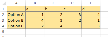
This example will let the viewer select from among the three options in this table.

Construction

Start by moving the original data range (shaded orange) down several rows, out of the way of the chart. This data can actually be located far away, even on another sheet.

Insert a “staging area” (shaded green below) and insert some temporary dummy data. This area can also be located anywhere else.

Create a chart using this staging area as its data source, and position it where desired.

You need to make the Developer tab visible in the ribbon, if it isn’t already. In Excel 2010 and 2013, click the File tab, click Options, click on Customize Ribbon, and in the right-hand list, check the box in front of Developer, and click OK.

On the Developer tab, click Insert, then in the Form Control section of the dropdown, click on the Combo Box button (second from left in first row).

The cursor turns into drawing crosshairs. Draw the Combo Box, then position it where you need it.

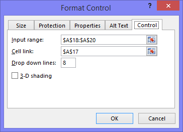
Right click on the Combo Box control, and choose Format Control. Click in the Input Range box, then select the range of cells that contains the items to show in the list (A18:A20). Click in the Cell Link box, and select the cell where the index of the selected list item will be displayed (A17). Click OK.

Write formulas in the green-shaded staging area. Select A15:E15, with A15 being the active cell, enter the following formula, then hold Ctrl while pressing Enter, to enter this formula into all of the selected cells:

=INDEX(A18:A20,$A17)

Note that the Combo Box control’s link cell is shaded blue in the screenshot below.

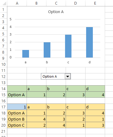
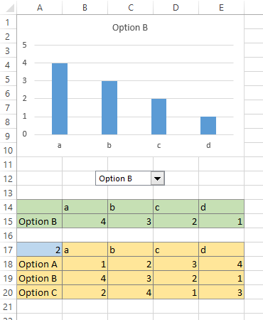
The interactive chart is now live. When you select another item in the Combo Box, the data in the staging area updates, and the chart displays the new data.

Options

You could just as easily use this interactive technique with a line chart, or pretty much any chart type.

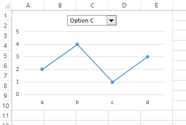
You also can locate the Combo Box control wherever you want. In the example below, it has been placed over the chart, taking the place of the chart title.

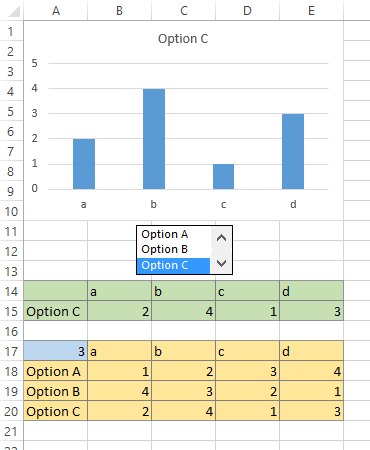
You are not constrained to using Combo Box controls. You could insert a List Box control (fifth button in the first row of the Insert Form Control dropdown on the Developer ribbon tab).

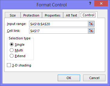
The format dialog for the List Box control is essentially the same as for the combo box, with an Input Range for the cells containing the items in the list, and a Cell Link for the cell displaying the selected option.

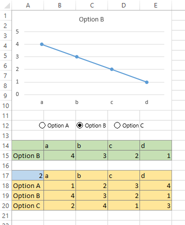
You could also use a series of Option Buttons (last button in the top row of the Insert Form Control dropdown on the Developer ribbon tab).

The format dialog for the Option Buttons only has a Cell Link box for the cell that indicates which option button is selected. You only need to format one Option Button in the set, though there is no Input Range, so the caption of each Option Button must be typed individually.

There are pros and cons of each of the control types used in this example.

The Combo Box is most compact, but only shows the selected item

The List Box shows all items in the list, but requires a space tall enough to display them all.

The Option Buttons show all items, and requires enough space for all Option Buttons needed. But these controls may be arranged in a column, or in a row, or in whatever arrangement you want.

Interesting Control Behavior

We already know that changing the control changes the Cell Link value, and therefore the staging area data and chart update. But typing a number manually into the Cell Link changes the staging area and chart, and also changes the control.

And if for some reason you have multiple controls that use the same Cell Link, changing any one control changes all of the controls as well as the staging data and chart.

This can be useful if you have several sheets of interactive charts, and you want all of the charts to show the same option. Set up only one Cell Link, on only one sheet, and use this Cell Link for all controls, and use its address in the formulas of all staging areas.