I’ve posted several examples of manipulating pivot tables with VBA, for example, Dynamic Chart using Pivot Table and VBA and Update Regular Chart when Pivot Table Updates. These examples included specific procedures, and the emphasis was on the results of the manipulation.
I thought it would be helpful to show some of the mechanics of programming with pivot tables. One important part of this is referencing the various ranges within a pivot table by their special VBA range names (which are actually properties of the Pivot Table object).
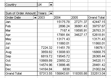
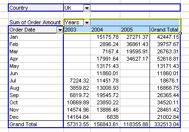
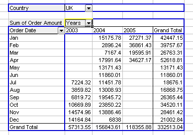
I’ll illustrate these special ranges using this simple pivot table, which comes from an example formerly available on the Microsoft web site (I can no longer locate it).
In VBA, you can reference a pivot table using this code in a procedure:
Dim pt As PivotTable
Set pt = ActiveSheet.PivotTables(1)
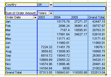
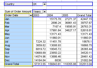
I’ve highlighted the various ranges using the indicated VBA commands.
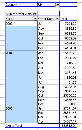
TableRange1
pt.TableRange1.Select
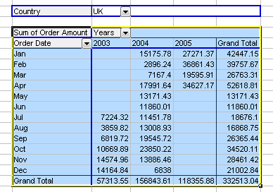
TableRange2
pt.TableRange2.Select
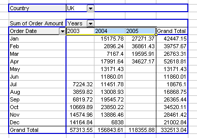
RowRange
pt.RowRange.Select
ColumnRange
pt.ColumnRange.Select
DataLabelRange
pt.DataLabelRange.Select
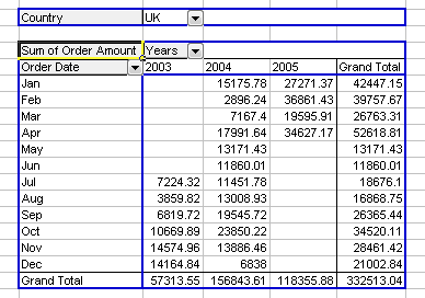
DataBodyRange
pt.DataBodyRange.Select
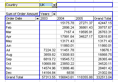
PageRange
pt.PageRange.Select
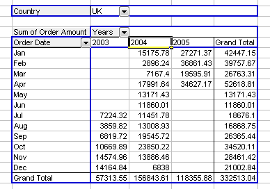
Pivot Field LabelRange
pt.PivotFields("Years").LabelRange.Select
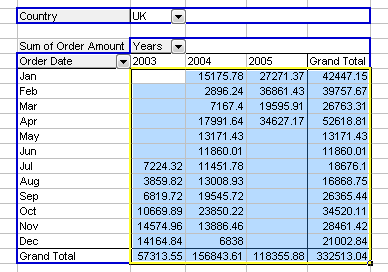
PivotField DataRange
pt.PivotFields("Years").DataRange.Select
Pivot Item LabelRange
pt.PivotFields("Years").PivotItems("2004").LabelRange.Select
Pivot Item DataRange
pt.PivotFields("Years").PivotItems("2004").DataRange.Select
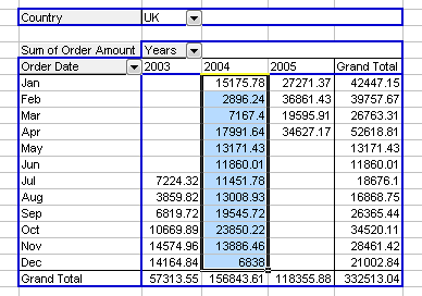
pt.PivotFields("Order Date").PivotItems("Feb").DataRange.Select

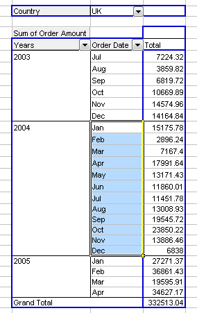
Pivot Field DataRange
The next few examples show the same ranges as above, after pivoting the table’s Years field from the columns area to the rows area.
pt.PivotFields("Years").DataRange.Select
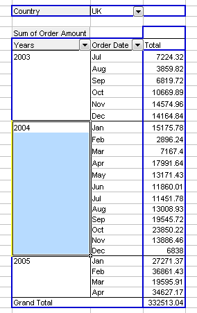
Pivot Item LabelRange
pt.PivotFields("Years").PivotItems("2004").LabelRange.Select
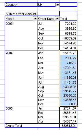
Pivot Item DataRange
pt.PivotFields("Years").PivotItems("2004").DataRange.Select
Complex Range
If a particular range isn’t specifically defined with a VBA property, you can use VBA range-extending properties EntireColumn and EntireRow and range operators Union and Intersect to define the range. For example:
Intersect(pt.PivotFields("Years").Pivotitems("2004").DataRange.EntireRow, pt.PivotFields("Order Date").DataRange).Select
Update
A follow-up post shows how to use this new skill to Create and Update a Chart Using Only Part of a Pivot Table’s Data.


Jeff Weir says
Jon…this is an outstanding tutorial, even by your standards. Thank you, thank you, thank you.
This alone is worth the price of the several excel reporting and charting books I purchased that – rather annoyingly – don’t have this essential charting info in them.
Colin Banfield says
An VBA object list described solely by visual worksheet examples. I’ve never seen a presentation quite like this. I think you’re on to something good here.
Jon Peltier says
Jeff & Colin –
When I went through this myself the first couple dozen times, I’d go to the Object Browser, read what it said, then when it wasn’t very clear, I’d run exactly the code I used here. Nothing like seeing something to understand it. Since few people are going to dig as deeply and obsessively as I did, it seemed like a good idea for a tutorial. If two smart guys like it, then I was on the right track.
AlexJ says
Jon,
Make it two and a half smart guys.
Doug Glancy says
Jon,
This is great. I’m sure I’ll refer back here again.
A few months ago I created a pivot table class, partly to teach myself this stuff. As part of it I created functions to return the row and column grand total ranges, because I didn’t see any vba properties for them. Here’s the on for the Row Grand Totals. It seems to work. What do you think?
Function RowGrandTotals() As Range
With pt
If .RowGrand = True Then
Set RowGrandTotals = .DataBodyRange.Offset(0, .DataBodyRange.Columns.Count – 1).Resize(.DataBodyRange.Rows.Count + (1 * .ColumnGrand = True), 1)
End If
End With
End Function
Jon Peltier says
Doug –
This works fine. Pretty much any range manipulation you can envision will be helpful. This article is to help people envision the pivot table structures in terms of properties of the Pivot Table object.
Jeff Weir says
Hi Jon. I’ve a couple of questions for you re this post.
1. Where you have “Dim pt As Pivot Table” above, should this be “Dim pt As PivotTable” (i.e. PivotTable is one word with no space between Pivot and Table)?
In 2007 I need to take the space out to get your code to work.
2. In the case that you have the Pivottable’s Years field in the columns area, how would you select say the readins for Feb only for the years 2003 – 2005?
3. I have fields formatted as date/time information across the top of my pivottabel, and I amend your code accordingly, I get an error “Unable to get the PivotItems property of the PivotField class”. That is, your code can handle columns that are formatted as text, or even numbers that are formatted as text, but not numbers or dates formatted as dates.
For instance, The code works if I rename the pivot columns as text such as “a”, which obviously forces Excel to treat it as text which your vba can handle.
For instance, the SQL query that populates the pivot table shows a certain date as “1/11/2008 00:00” (when viewing the raw SQL output in SQL Query Analyzer). My pivot table formats this as “1/11/2008”. But I get an error if I use a VBA statement like this:
pt.PivotFields(“Order Month/Year”).PivotItems(“1/11/2008 00:00”).DataRange.Select
…or this:
pt.PivotFields(“Order Month/Year”).PivotItems(“1/11/2008”).DataRange.Select
…or this:
pt.PivotFields(“Order Month/Year”).PivotItems(“39753”).DataRange.Select
However, if I overtype the field as something like “a” then this works:
pt.PivotFields(“Order Month/Year”).PivotItems(“a”).DataRange.Select
…and if I overtype the field as “1/11/2008” (which sticks it in as text, not as a date) then this works:
pt.PivotFields(“Order Month/Year”).PivotItems(“a”).DataRange.Select
…and in both these cases, what I type in is automatically left-aligned as opposed to the original pivotfields, which are all right-aligned.
Interestingly, if I overtype 1/11/2008 with the number equivalent 39753, Excel doesn’t format it as text and the code fails. But if I then overtype 39753 with “a”, and then overtype “a” with 39753, excel treats it as text and the code works.
I take it from this that I need to amend the VBA in some way to tell it i’m looking for date/time information, not searching for text. Do you have any idea if this is the case, and if so, what kind of statement I need?
Thanks for any help.
Jeff
Jon Peltier says
Jeff –
1. Yes, there is no space in PivotTable, good catch.
2. pt.PivotFields(“Order Date”).PivotItems(“Feb”).DataRange.Select
3. What I generally do is loop through the pivot items, and compare the pivot item caption to what I’m looking for:
For Each pi In pt.PivotFields("Order Month/Year").PivotItems
  If pi.Caption = Format(TheDate, "m/dd/yyyy") Then
  ' or If DateValue(pi.Caption) = TheDate Then
    '' FOUND IT
  End If
Next
Jeff Weir says
Hi Jon. That’s great. Sorry, 2 more questions for you on this. (You are probably going to cringe when you see how little I understand of VBA…I’m still working my way though Walkenbach’s Power Programming).
1. Once I’ve used the loop you’ve posted above in answer to my last question, how do I then select the PivotItem concerned? For instance, I tried each of the following modifications to no avail (put them in the THEN part of your code) :
pt.PivotFields(“Order Month/Year”).PivotItems(Format(“1/1/2009”, “m/dd/yyyy”)).DataRange.Select
pt.PivotFields(“Order Month/Year”).PivotItems(Pi.Caption).DataRange.Select
pt.PivotFields(“Order Month/Year”).PivotItem.DataRange.Select
2. In your example, how would I modify pt.PivotFields(”Order Date”).PivotItems(”Feb”).DataRange.Select
to select say Feb’s figure for 2004 and 2005, but not 2003?
This gives me Feb’s figure for 2004:
Intersect(pt.PivotFields(“Order Date”).PivotItems(“Feb”).DataRange, pt.PivotFields(“Years”).PivotItems(“2004”).DataRange).Select
But I cant’ simply add in another year like this:
Intersect(pt.PivotFields(“Order Date”).PivotItems(“Feb”).DataRange, pt.PivotFields(“Years”).PivotItems(“2004″,”2005”).DataRange).Select
…as I get the error “Wrong number of arguements or invalid property assignment”
Sorry for the stream of questions.
Regards, Jeff
Jon Peltier says
1. Here’s what I had in mind:
For Each pi In pt.PivotFields("Order Month/Year").PivotItems
  If pi.Caption = Format(TheDate, "m/dd/yyyy") Then
  ' or If DateValue(pi.Caption) = TheDate Then
    pi.Select
    Exit For
  End If
Next
2. To select the data for 2004 and 2005, you would use something like this:
Union(pt.PivotFields("Years").PivotItems("2004").DataRange, _
    pt.PivotFields("Years").PivotItems("2005").DataRange).Select
So the Feb data for these two years would be
Intersect(pt.PivotFields("Order Date").PivotItems("Feb").DataRange, _
    Union(pt.PivotFields("Years").PivotItems("2004").DataRange, _
    pt.PivotFields("Years").PivotItems("2005").DataRange)).Select
Keep in mind that you do not need to select something if you just need to extract the data.
Jeff Weir says
Thanks Jon. Awesome.
LEM says
Hey Jon,
Is there a way to apply a conditional format to a Pivot Table that would Bold Font and Highlight in Yellow entire rows that have met a certain condition in one of the columns?
Thank you!
Jon Peltier says
You can use the same conditional formula as you would with a worksheet range (non-pivot). If the pivot table resizes, you’ll have to reapply or remove the conditional formatting, but if the pivot table refreshes without resizing, the conditional formatting works fine.
LEM says
Hmmmm… Interesting, because when I refresh my pivot it will keep the conditional format on the first three columns, but the rest of the columns will lose the format when it is refreshed. Then if I try to Apply it again it does not work, and I have to re-enter the formula. The Pivot Table is not ‘resizing’ due to a filter for the Top 100 Items… So I was hoping there was some way to automate this…
Thanks again for the help!
Jon Peltier says
I tested in Excel 2003 SP3, and the pivot table had three row fields and one data field. The data came from a list (“table” in 2007) and the data field values were volatile random numbers. Pressing F9 then refreshing the pivot table resulted in the formats updating to reflect the new values.
LEM says
Sorry I keep having to post…
I am in Exel 2007, and my List Data is on a separate tab, I have the following in my PivotTable Field List:
1 Report Filter
2 Column Labels (One of which is ‘Values’ from the last Field List box)
3 Row Labels
9 Values
Even when I try pressing F9 (?) and refresh it will drop columns (from =$B$10:$V$109 to =$B$10:$D$109. (Only formatting my Row Labels, and losing formatting on all of the Values.
Because of this I was hoping I could include something within a Macro (that currently just does small things like column size adjustment) that would also update the conditional format Applied To Range.
Hope this makes sense :)
LEM says
Just to add to the above:
And anytime I try to just ‘record’ my actions for conditional formatting nothing shows up…
Jon Peltier says
I haven’t used conditional formatting much in 2007, and I haven’t programmed conditional formatting much in any version.
You could just do a generic formatting routine, following this pseudo-code:
for each row in pivottable-pivotfield-datarange-rows
..if row.cells(1,1).value > threshold value then
….row-entire row of pivot table-format-color and bold
..else
….row-entire row of pivot table-format-plain
..end if
next
LEM says
I would like to apologize in advance (and thank you for your patience!), because I am still very much a beginner in coding and trying to learn … But I am not sure exactly what to do… So far:
Sub PivotConditionalFormat()
‘
‘ PivotConditionalFormat Macro
‘
‘Bold and Highlight
pt.TableRange1.Select
Selection.FormatConditions.Delete
Selection.FormatConditions.Add Type:=xlExpression, Formula1:C =”=IF(C=”TEXT”,TRUE,FALSE)”
With Selection.FormatConditions(1).Font
.Bold = True
.ColorIndex = 3
End With
End Sub
But of course nothing works… I get errors thrown up all around the Formula and cannot get past this to even try it out – or see what other errors I have
Jon Peltier says
LEM –
If you have to use VBA to reapply conditional formatting every time the pivot table is refreshed, you might as well take the easy way out, skip the conditional formatting, and apply the formatting directly in the VBA routine. I’ve written up an example in Pivot Table Conditional Formatting with VBA. Thanks for the blog topic.
Si says
Hi Jon
Very useful post,
A quick question if I may, I am using your code to automate the formatting of a set of sheets with pivot tables, all of which are different . My aim is to open a the workbook, change the source data for the day click refresh all pivots and have all the pivots format themselves.
I have been using the below code to format all the pivot tables.
Sub Format_Pivots()
Dim PT As PivotTable
Dim ws As Worksheet
Dim wb As Workbook
Set wb = ActiveWorkbook
For Each ws In Worksheets
For Each PT In ws.PivotTables
With PT.TableRange1
.Borders(xlInsideVertical).LineStyle = xlContinuous
.Borders(xlInsideHorizontal).Weight = xlContinuous
.Borders(xlEdgeTop).LineStyle = xlContinuous
.Borders(xlEdgeLeft).LineStyle = xlContinuous
.Borders(xlEdgeRight).LineStyle = xlContinuous
.Borders(xlEdgeBottom).LineStyle = xlContinuous
.Borders(xlEdgeTop).LineStyle = xlContinuous
.Borders(xlEdgeBottom).LineStyle = xlContinuous
.Borders(xlEdgeLeft).LineStyle = xlContinuous
.Borders(xlEdgeRight).LineStyle = xlContinuous
End With
Next PT
If Not (wb.Name Like “5 Week PTL*”) Then
ws.Columns(“B:Z”).ColumnWidth = 8.14
ElseIf Not (wb.Name Like “Obstetrics Waiting List*”) Then
ws.Columns(“B:Z”).ColumnWidth = 8.14
Else
ws.Columns(“C:Z”).ColumnWidth = 8.14
End If
Next ws
End Sub
However when I use pt.ColumnRange.Select & pt.DataBodyRange.Select I cannot get it to work unless I use your code specifying pivot table 1.
What am I missing?
Jon Peltier says
Si –
1. You’ve neglected to say which version of Excel you are using.
2. I see no references to ColumnRange or DataBodyRange in the code.
3. I removed the ColumnWidth stuff, and the rest of your code ran just fine in Excel 2003.
Rupert says
Hi,
I was wondering if you know how to add comments to a pivot table via VBA.
I have data in a worksheet in the following format :
SalesStation,Date,Value,Comments
S01,01/10/2009,100
S01,02/10/2009,150,low sales on this day
S01,03/10/2009,120
and I would like to add any comments to the data field as a little red marker in the top right corner of the cell if there is a comment for that value.
Thanks
Jon Peltier says
Rupert –
Like all expert VBA programmers, I considered your question, then fired up the macro recorder while adding a random comment to a random cell. Here is what it told me:
Sub AddComment()
'
' AddComment Macro
' Macro recorded 10/27/2009 by Jon Peltier
'

'
    Range("H6").AddComment
    Range("H6").Comment.Visible = False
    Range("H6").Comment.Text Text:="Jon Peltier:" & Chr(10) & "Low sales on this day"
End Sub
I trimmed the code to:
Sub AddCustomComment()
'
' AddComment Macro
' Macro recorded 10/27/2009 by Jon Peltier
'

'
    Range("H7").AddComment.Text Text:="Low sales on this day"
End Sub
It’s up to your code to identify the cell that should get the comment, and to remove comments when they are no longer applicable.
Rupert says
Thanks John,
This is what I have so far :
Private Sub addcomments(sheetname, pivottablename)
Dim c As Range, pvtitem As PivotItem, d As Range
With Sheets(sheetname).PivotTables(pivottablename)
If .RowRange.Count > 2 Then
For Each c In .PivotFields(“count of comments”).DataRange.Cells
If c.Value = 1 Then
Set d = Cells(c.Row, c.Column – 1)
d.AddComment “test”
Else
End If
Next
Else
End If
End With
End Sub
I can identify which cell to add the comment to but the problem is getting the text form the comments field actually into the d.addcomment “test” part above.
Do you have any ideas for it?
Thanks,
Rupert
Jon Peltier says
Rupert – Are the comments visible in the pivot table?
Rupert says
Yes, I get a comment in the cell.
The problems are :
1) I have to add the comments field as a data field – “count of comments” – and do a count on it so it is visible.
I then have to add a comment to the same row, previous column in the value data field if a value exists in the “count of comments” data field, and then hide the “countof comments” data field.
2) i cant seem to extract the actual comments text from the comments field into the inserted comment in the value data field.
Let me know if you want me to send a sample to you.
Cheers,
Rupert
Jon Peltier says
I’m thinking that putting the comments field into the rows area might help…
Rupert says
Hi Jon,
Think I’ve got it. Heres what I did :
Sub insertcomments(sheetname, pipelinecode, processplantname, _
                   SalesStationCode, pivottablename)
  Dim datarange As Range, commentsrange As Range, custcode As Range
  Dim pprange As Range, ssrange As Range, catrange As Range, piperange As Range
  Dim d As Integer, mynames() As String
  Dim cust As String, datefield As String, pp As String
  Dim SSCode As String, cat As String, pipecode As String
  Dim pvtitem As PivotItem

  Worksheets("qryexcelexport").Select
  Set datarange = ActiveSheet.Range("A1").CurrentRegion
  ReDim mynames(datarange.Columns.Count)

  For c = 1 To datarange.Columns.Count
    mynames(c) = Cells(1, c).Value
  Next

  d = datarange.Rows.Count
  On Error Resume Next
  For e = 2 To d
    If Not IsEmpty(Cells(e, c - 1)) Then
      For f = 1 To c - 1
        Select Case mynames(f)
          Case "processPlantName"
            pp = Cells(e, f).Value
            Set pprange = Sheets(sheetname).PivotTables(pivottablename) _
                          .PivotFields("processPlantName").PivotItems(pp).datarange
          Case "SalesStationCode"
            SSCode = Cells(e, f).Value
            Set ssrange = Sheets(sheetname).PivotTables(pivottablename) _
                          .PivotFields("SalesStationCode").PivotItems(SSCode).datarange
          Case "CustomerCode"
            cust = Cells(e, f).Value
            Set custcode = Sheets(sheetname).PivotTables(pivottablename) _
                           .PivotFields("CustomerCode").PivotItems(cust).datarange
          Case "Category"
            cat = Cells(e, f).Value
            Set catrange = Sheets(sheetname).PivotTables(pivottablename) _
                           .PivotFields("Category").PivotItems(cat).datarange
          Case "PipelineCode"
            pipecode = Cells(e, f).Value
            Set piperange = Sheets(sheetname).PivotTables(pivottablename) _
                            .PivotFields("PipelineCode").PivotItems(pipecode).datarange
          Case "Date"
            datefield = Format(CDate(Cells(e, f).Value), "m/d/yyyy")
            Set daterange = Sheets(sheetname).PivotTables(pivottablename) _
                            .PivotFields("Date").PivotItems(datefield).datarange
          Case Else
        End Select
      Next

      With Sheets(sheetname).PivotTables(pivottablename)
        Set commentsrange = Intersect(pprange, ssrange, custcode, _
                                      catrange, piperange, daterange)
        commentsrange.AddComment Cells(e, c - 1).Value
      End With
    End If

    Set pprange = Nothing
    Set ssrange = Nothing
    Set custcode = Nothing
    Set catrange = Nothing
    Set piperange = Nothing
    Set daterange = Nothing
    Set commentsrange = Nothing
  Next

End Sub
Thanks for your time anyway, Rupert
Final Impact says
Hi Jon and thanks for the above info it was helpful and insightful!
I am however at a loss as to how to do something simple and use cells from a sheets range like f2 to f32 to make items in a Pivot field ‘PivotItems Visible = True’. I’ve recorded macros and attempted to automate the process but I’m missing something. (Too many problems to list)
The PT comes from a table of test records with 30 columns and 15k rows. My PT is setup but I have to manually uncheck “Show All” and search for and check-off 200 serial numbers in column 1 of the PT every three days.
Can I point my vb code to a list or range cells and exclude everything in the column which is not in the column I specifiy (f2:f32 or A1 to A201) from another sheet?
PT headers are as follows: SERIAL_NUM, CAL_DATE, CAL_TIME, SLOT, ERROR_MESS, ect. and all I need is SERIAL_NUM visible equal to true for 200 of the 15k serial numbers available. Does this make sense?
Thanks for any input.
Final Impact
Fernando says
dear:
In your article you datarange reference data, as I do to reference a data item in the grand total column using de intersect property:
in the example
pt.DataBodyRange.Select
as I do to select in the row
Order Date “Jan” Grand Total “42447,15”
this cell is not inside in the datarange ?.
as do I reference the column grand total ?
thanks you very much
Craig says
Jon this is quite a useful article. Definitely the closest thing I’ve found to what I’m looking for. I was hoping this might be an appropriate place to take me the last step.
I see above that using VBA, there are easy ways to return whole ranges from a pivot table that will dynamically resize. However, is there a way to fetch a pivot table range from a formula that might reside on another worksheet? Basically, I have two separate pivot tables that contain some different data. I also have some formulas on another worksheet that reference ranges in both of these tables to do some calculations; for example, one of my formulas would include LINEST(). In my formulas, I would like to reference the pivot table ranges, which may change as I manipulate what’s displayed on the pivot table. Is this possible to do with formulas? All I can find so far is the GETPIVOTDATA() function, but the documentation indicates that this is only for the summary data, whereas I want to operate on the range itself.
Regards,
Craig
Jon Peltier says
Hi Craig –
I think this could be done with UDFs. One approach is to create a UDF like this (untested):
You could then call it like:
Craig says
Hmm, that is an interesting way of approaching this problem, and one that I had not considered before. I’ll give it a shot and let you know if it works. The concept seems like it should, though.
Thanks a lot!
Gaetan says
Great post, extremely useful as an introduction.
Question :
When you have two calculations, we then have a pivot field names “data” (données in french). In order to keep international compatiblity, do you know a way to capture the range of this cell.
Thanks a lot.
Jon Peltier says
Gaetan –
Instead of searching for each pivot field in YourPivotTable.PivotFields, try one of these:
For Each PvtFld In YourPivotTable.PageFields
For Each PvtFld In YourPivotTable.RowFields
For Each PvtFld In YourPivotTable.ColumnFields
For Each PvtFld In YourPivotTable.DataFields
Gaetan says
Jon –
I think I should only look at rowfield and columnfield for “data” as I don’t think “data” could be a datafields, neither could be a pagefield.
That said, as I don’t know in advance what will be the orientation of the data, I preffer to scan every possibility (I guess this could be specific to my problem).
Beside the speed, do you see any other inconvenient?
Thank you for your answer.
Gaetan
Jon Peltier says
Gaetan –
In general there isn’t any real inconvenience to cycling through items in VBA. The computer does it behind the scenes, and if there isn’t a huge number of items, the user will not notice.
Gaetan says
That’s what I was thinking.
Thanks for confirming.
Gaetan
Robert - Norwalk, Connecticut says
I made good use of your Pivot calls for vba above. I tried getting the “Grand Total” field and failed using pt.PivotFields(“Years”).PivotItems(“Grand total”).DataRange.Select. Is there something different about that column.
Sorry, I may have missed something.
Thanks
Jon Peltier says
Robert –
The totals are not distinct fields, but are part of the DataBodyRange, if the totals are included in the table. The code below bolds the column of row totals, italicizes the row of column totals, and shades the grand totals light gray. The grand total will be bold and italic, since it’s in the row totals and column totals.
Michael Daly says
Hi Jon
Excellent article, but could you give me the equivalent way to reference PivotTable properties in MS Access (say 2003 or 2007)? I am trying to change the ‘Fill color’ property of a ColumnAxis field using VBA.
I can update the ‘Caption’ property, but I just can’t crack how to update the Backcolor or Fill color property using this code:
The next line works…
Me.PivotTable.ActiveView.ColumnAxis.FieldSets(0).Fields(0).Caption = “Event”
The next line doesn’t work.
Me.PivotTable.ActiveView.ColumnAxis.FieldSets(0).Fields(0).FillColor = vbYellow
Nor this line…
Me.PivotTable.ActiveView.PivotFields(0).FillColor = vbYellow
I have tried FillColor, BackColor, SubtotalBackcolor, but I just can’t reference this object correctly. Do you know how to reference this object so I can update the ‘BackColour’ property with VBA?
I appreciate your help.
Michael Daly
29 April 2010
Jon Peltier says
Michael – You’ll have to ask someone who uses Access.
Akshat says
How can i change pagefield data of pivot using VBA
Jon Peltier says
Akshat –
To put a field into the page area:
To change which item appears in the page field:
Adam says
I’m trying to create multiple pivot tables using a pivot cache from another worksheet. I just keep modifying the same pitot, what am I missing?
Row = 1
For i = 1 To pf.PivotItems.Count
ItemName = pf.PivotItems(i)
Set PT = PTCache.CreatePivotTable _
(TableDestination:=RepSummary.Cells(Row, 1), _
TableName:=ItemName)
Row = Row + 30
‘Add fields to the new pivot
With PT.PivotFields(“SALESREP_NAME”)
.Orientation = xlRowField
.Caption = “Sales Rep”
End With
With PT.PivotFields(“Total”)
.Orientation = xlDataField
.Caption = “Volume ($)”
.Position = 1
.NumberFormat = “#,##0”
End With
With PT.PivotFields(“Uph”)
.Orientation = xlDataField
.Caption = “Uph Volume ($)”
.Function = xlSum
.NumberFormat = “#,##0”
End With
Jon Peltier says
Adam –
Have you defined PTCache?
When I do this manually, I copy the original pivot table, paste it where I want the new one, and modify the layout of the new pivot table. This might be easier in code as well.
Adam says
Jon:
I have: Set PTCache = ActiveWorkbook.PivotCaches(1) ‘where 1 is the original cache i wish to use.
I’ll try your idea of merely copying the table and then use the With command to alter the layout as you suggest.
The complication also arises in that i’m using the field values pf.PivotItems from the original pivot table to create 32 different (new) pivot tables in a new sheet.
I’ll let you know if the suggestion works out (i.e. if i’m smart enough to write the darn thing)…
-Adam
p.s. your visual tutorials are indeed helpful and will come in handy.
Tiffany says
This post is wonderfully helpful! I have a followup question: how do you reference data labels in a nested pivot table? For example I have a pivot table with two columns (number and percent) under each data label (original and revised).
Original | Revised
# | % # | %
How would I reference, for example, the # data label in the Revised column? I can select the Revised label via the below”
PivotFields(“Original or Revised”).PivotItems(“Revised”).LabelRange.Select
but I’m not sure how to select the sublabels, for lack of a better term. Hope that makes sense…looking forward to any guidance you can offer. Thanks!
Tiffany
Jon Peltier says
Adam – The macro recorder is your friend….
Jon Peltier says
Tiffany –
Can you use Intersect? In pseudo-code:
Adam says
Jon;
Quite true.
Found my error…incidentally it was very simple, the Row +30 wasn’t enough to allot for the new pivot. Now the code works. When all else seems right…it is…look for the simple things and most often that’s it.
Tiffany says
Intersect works perfectly, thanks!!!
Jeff Weir says
Jon…using Excel 2007, if I use pt.PivotFields(“Years”).LabelRange.Select then it just selects the header “Years”only from the pivot table and not the items underneath.
If I use pt.PivotFields(“Years”).PivotItems(“2004″).LabelRange.Select then I’ll get the 2004 items, same as you do.
Any idea how I select all the rows under a particular pivotfield? (and preferably not the heading itself)
Jon Peltier says
Jeff –
This might be a case where you have to build the range you want using Union() and Intersect().
Jeff Weir says
The problem was that the pt.RowRange.Select command (the way you are using it without the optional arguments) works differently for a pivot table constructed in excel 2007 than one constructed in excel 2003.
* In a pivottable created in excel 2007, if you don’t supply the optional arguments then the default is to just selects the headers.
*In a pivottable created in 2003, if you don’t supply the optional arguments this selects the headers and all the rows below. (note this happens for an excel 2003 pivottable that has been opened in excel 2007 too). Note that this is not what the help file says it does…the help file example supposedly selects just the row headers on the PivotTable report. Looks like an error that it’s working the way it is in 2003 to me.
RowRange takes 2 arguments…a rowindex number and a columnindex number. Then it works like an index function i.e. it drops down x rows according to the rowindex argument and across y columns according to your columnindex arguement.
So pt.RowRange(3,1) will select the cell two rows under the first column heading i.e. row 3, column 1. Note that pt.RowRange(3,10) will select a cell in the data area (because you only have 2 columns in this example, but you’ve asked excel to keep on heading west). So if you provide a columnindex number, this function doesn’t restrict you to returning cells from your row fields.
However, if you omit the columnindex and just use pt.RowRange(3) then excel starts counting cells from left to right, dropping down whenever it reaches the last column in the row area (in this case, column 2). So you’ll be selecting column 1, row 2 of the pivot table.
In any event, I think pt.RowRange.Select is not the right command to use if you want to select row columns as shown in your example above…certainly if your code might be used on an Excel 2007 pivottable. Instead, you should use pt.RowRange.Columns.Select
If you want the first column, then you should use pt.RowRange.Columns(1).Select or replace the 1 with the name of the column you want in speech marks e.g. “Years”
Jon Peltier says
Gee, an inconsistency between 2007 and 2003. 1/2 of my recent project work has been building ribbon interfaces for projects being upgraded to 2007, and another 1/4 has been finding and programming around such inconsistencies. It keeps the revenues coming in, but it’s not very challenging or interesting.
guti says
Hello Jon,
I am new to pivot tables so I found your post extremely helpful but I could really use your help solving a problem.
I am running MS excel 2003
I am trying to create reports for specified time periods which will be defined in two cells (one for the start date and the other the end date) by the users. I was hoping that the code below would achieve this but I get an error and usually only display the last date. I have even tried adding a false condition thinking that was missing but I still get errors. I really appreciate your time.
start_date = “E6”
end_date = “G6”
For Each pvtItem In ActiveSheet.PivotTables(“PivotTable3”).PivotFields(“Date”).VisibleItems
If (pvtItem.Name > end_date) Then
pvtItem.Visible = False
End If
Next pvtItem
Jon Peltier says
You have told VBA that the start and end dates are addresses E6 and G6, not the values in these cells. Use:
start_date = ActiveSheet.Range(“E6”).Value
end_date = ActiveSheet.Range(“G6”).Value
Nicholas says
Hi i got a project and i wish to know using the below code i will like to create using this method how to i get the cell range? if i can get this method i can then complete my project
pt.TableRange1.Select – getting a Range example A1:D8 something like that.
Jon Peltier says
Nicholas –
To get the range, use this syntax:
strAddress = pt.TableRange1.Address
Nicholas says
So does this also apply to the grand total at the bottom as i have to know the particular cell address for different column associated with it
Item | Example 1 | Example 2|
Item1 | 2 | 3 |
Item2 | 5 | 2 |
Grand Total | 7 | 5 | <– Using this column to convert into the below
Item | Example 1 | Example 2|
Grand Total | 7 | 5 |
Due to the changes in the raw data and there are many of such pivot tables with different conditions and the process required after that i cant just create another pivot table with the condition i want.
Jon Peltier says
Nicholas – I don’t understand. Could you explain in a bit more detail?
Nicholas says
Sorry, i will like to make individual Charts of the Pivot table and as well as a overall View.
Image 1 – My Data – http://yfrog.com/mc74482374p
Image 2 – My Pivot Tables – http://yfrog.com/8644108178p
Image 3 – My Overall Table – http://yfrog.com/bh15920375p
In my Overall Table i am required to update the Grand Total For each category( which is Example 1 to Example 4 as shown on my Data) and i have about 2 – 3 different Overall Tables so with different combination and after that i required to do a chart and also using the chart i need to do many other function which by using pivot table i am unable to access.
I also need to produce a chart of different Category(from example 1 to example 4)
its something like that. sorry to trouble you.
Jon Peltier says
Nicholas –
If your data were shaped differently, it would be easy with another pivot table and without code. Keep columns A through E as is, put the example label in column F, and put the True/False in column G. You will have four rows per S/N with the other data repeated in the new rows. This way, you could put column F into the rows area of the pivot table, Column G into the columns area and into the data area, to get your summary.
If the hidden label for the rows area is “Class”, you can also get your pivot tables from the new data arrangement: put Example (column F) in the page area, and column G in the data area and in the columns area, and Class in the rows area.
Dan Shedd says
this is a great post, i only wish i had found it sooner. i used the macro recorder to figure out how to change the date format of a pivot field, and since it was a row field i was changeing the macro recorder used the .Name proprty. Unfortunately when you put this in a VBA script it doesn’t change the date format of the pivot item it actually changes the name of the pivot field! i found some reference to .NumberFormat but according to MS documentation it only is for data fields. I tried it for a row field and it works anyway
With .PivotFields(“Service_Date_From”)
.Orientation = xlRowField
.Subtotals = Array(False, False, False, False, False, False, False, False, False, False, False, False)
.NumberFormat = “m/d/yyyy”
End With
Here’s the M$ article
“You can set the NumberFormat property only for a data field.”
excel seems to be very picky, any other date format and the intersection command fails
unless i am doing something really wrong here
JonV says
Hi Jon,
Thanks – this site is a great reference. My quest is regarding Grand totals. Your reply to Robert with “Sub SelectGrandTotal()” helped “break the logjam” for me.
I did arrive at a solution. However, it seems inelegant (and isn’t elegance in coding what we’re all after? 8^).
Using your above PT example, I’ve been trying to grab specific Grand Total values.
For instance, to get the Grand total for 2004 (a value of $156843.61) I arrived at the following structure:
Again, is there a better way to get ‘sDataValue’ with having to resort to row/column matrixing/intersecting?
Thanks much!
JonV
Jon Peltier says
Let me preface my reply by pointing out that elegance in code is overrated. Now, if it works, that’s elegant enough.
I think I may have done something like this, pending a few tests to make sure it’s going to work:
sDataValue = intersect(pvtitem.datarange.entirecolumn, rcolumntotal.entirerow).value
Whether it’s more or less “elegant”, I don’t know. I didn’t bother to fill out the whole sub, so I can’t even gloat about mine being done in fewer lines.
JonV says
Thanks – thats much cleaner.
I’ll run with this structure:
Hey – one less variable – thats elegant!
JonV
Jim Lovejoy says
Hi Jon, excellent write up. Used most of your you posted code for formatting Grand Totals above, but I’m having trouble finding how to get to the totals in column L. Hoping you might point me in the right direction.
I can’t seem to get to anything in column L, Label or Data Ranges. Also, I’m not able to find a way to alternate the colors of the drives as shown above. I’ve tried everything, and all I can get is all drives as one color.
Any help will be greatly appreciated. – Thanks (Excel 2003, and 2007)
http://cid-82a2b12e3596784a.office.live.com/self.aspx/.Public/Drives.jpg
With pt
If .ColumnGrand And .RowGrand Then
With .DataBodyRange ‘ Unknown
Set rGrandTotal = .Cells(.Rows.Count, .Columns.Count)
rGrandTotal.Interior.ColorIndex = 2
rGrandTotal.Font.ColorIndex = 1
End With
End If
If .ColumnGrand Then
With .DataBodyRange ‘Row All Grand Total (Bottom)
Set rColumnTotal = .Rows(.Rows.Count)
rColumnTotal.Interior.ColorIndex = 1
rColumnTotal.Font.ColorIndex = 2
rColumnTotal.Font.Italic = True
rColumnTotal.ColumnWidth = 7.71
End With
End If
If .RowGrand Then
With .DataBodyRange ‘Virtical SAN Grand Total
Set rRowTotal = .Columns(.Columns.Count)
rRowTotal.Interior.ColorIndex = 1
rRowTotal.Font.ColorIndex = 2
rRowTotal.Font.Bold = True
rRowTotal.ColumnWidth = 7.71
End With
End If
With .PivotFields(“Drive”).LabelRange.Select
Selection.Interior.ColorIndex = 1
Selection.Font.ColorIndex = 1
End With
With .PivotFields(“Drive”).DataRange.Select
Selection.ColumnWidth = 5.86
Selection.Interior.ColorIndex = 15
Selection.Font.ColorIndex = 1
End With
With .PivotFields(“LOCAL”).LabelRange.Select
‘Selection.ColumnWidth = 5.86
Selection.Interior.ColorIndex = 35
Selection.Font.ColorIndex = 1
End With
With .PivotFields(“LOCAL”).DataRange.Select
Selection.Interior.ColorIndex = 35
Selection.Font.ColorIndex = 1
End With
With .PivotFields(“SAN”).LabelRange.Select
Selection.ColumnWidth = 5.86
Selection.Interior.ColorIndex = 19
Selection.Font.ColorIndex = 1
End With
With .PivotFields(“SAN”).DataRange.Select
Selection.Interior.ColorIndex = 19
Selection.Font.ColorIndex = 1
End With
Jon Peltier says
To get the total of one of the column fields, you need to determine how many column fields there are, and the index of the desired column field among all column fields. There are as many column field totals as column fields, and the index of the total is the same as of the column field. Lots of intersect-type range definition.
You’ve defined colors for the LOCAL and SAN parts of each drive. To define individual colors for each drive’s LOCAL and SAN data, you’ll need to use Intersect(Drive, Data) to identify the range.
Orison says
Hi Jon, please i need you help
i have this code:
Range(“IO17”).Select
ActiveSheet.PivotTableWizard SourceType:=xlDatabase, SourceData:= _
“Despiece!R4C1:R3000C45”
‘ActiveSheet.PivotTables(“Tabla dinámica1”).RefreshTable
Dim ThisPage As String
PageField1 = ActiveSheet.PivotTables(“Tabla dinámica1”).PivotFields(1)
OrigPage = ActiveSheet.PivotTables(“Tabla dinámica1”).PivotFields(PageField1).CurrentPage
NumPages = ActiveSheet.PivotTables(“Tabla dinámica1”).PivotFields(PageField1).PivotItems.Count
For j = 1 To NumPages
ThisPage = ActiveSheet.PivotTables(“Tabla dinámica1”).PivotFields(PageField1).PivotItems(j)
If ThisPage = FrmDespachos.SpreadDes.Cells(i + 1, 1).Text Then
ActiveSheet.PivotTables(“Tabla dinámica1”).PivotFields(PageField1).CurrentPage = “(All)”
ActiveSheet.PivotTables(“Tabla dinámica1”).PivotFields(PageField1).CurrentPage = ThisPage
ERROR 13 error 13 Type Mismatch
ERROR 13 error 13 Type Mismatch
‘ActiveWindow.SelectedSheets.PrintOut
End If
Next j
‘ActiveSheet.PivotTables(“Tabla dinámica1”).PivotFields(“DESP.”). _
CurrentPage = FrmDespachos.SpreadDes.Cells(i + 1, 1).Text
I found the error but still can not find the solution, the problem is that when I load my PivotTable refresh data then does not take a fact as the first element to be filtered, in office 2000 after loading the data (there this in my code) has already leaked the PSED data. = “0003” but in 2007 this office DESP .= “All”
Is there any way that my pivot table after load data is selected filter element and is not in “All”
Regards
Orison
From Lima Peru :)
Jon Peltier says
Don’t leave off the properties of the various objects. The default property may not be what you expect.
ActiveSheet.PivotTables(“Tabla dinámica1″).PivotFields(1).Caption
ActiveSheet.PivotTables(“Tabla dinámica1″).PivotFields(PageField1).CurrentPage.Name
ActiveSheet.PivotTables(“Tabla dinámica1″).PivotFields(PageField1).PivotItems(j).Caption
Also, CurrentPage is not defined if the PivotField is not a page field?
Orison says
Thanks, i have a solution :)
***********************************
With ActiveSheet.PivotTables(“Tabla dinámica1”).PivotFields(“DESP.”)
.PivotItems(strDespacho).Visible = True
End With
************************************************
Now i hace new problem with this code :
***************************************************
Sheets(“FORMAS”).Select
Range(“A1”).Select
Selection.PasteSpecial Paste:=xlValues, Operation:=xlNone, SkipBlanks:= _
False, Transpose:=False
‘LENTO
Selection.PasteSpecial Paste:=xlFormats, Operation:=xlNone, SkipBlanks:= _
False, Transpose:=False
ActiveWindow.Zoom = 75
the problem is that when you copy data to another excel sheet everything is perfect copy raw data, then copy the format for the 19 entries, but I see the excel as having selected or openness, but plain cells but is selected as 1046215 incredible, so in this line of paste forms takes too long and slows the process. In Office 2000 is fast I have no problems but it is slow in Office 2007. You know that is?
Thank you.
Orison
***********************************************************
Jon Peltier says
Orison – What did you copy?
Orison says
Hi Jon
My code to copy is:
*********************************************************************
Range(“A2”).Select
Selection.Sort Key1:=Range(“A2”), Order1:=xlAscending, Key2:=Range(“F2”) _
, Order2:=xlAscending, Key3:=Range(“G2”), Order3:=xlAscending, Header:= _
xlGuess, OrderCustom:=1, MatchCase:=False, Orientation:=xlTopToBottom
Selection.AutoFilter
Range(“A2”).Select
Selection.AutoFilter Field:=1, Criteria1:=DESPACHO
Columns(“A:AB”).Select
Selection.Copy
Windows(Name & “.xlsx”).Activate
Only copy 20 Rows.
Thanks.
Orison
Jon Peltier says
Orison –
You say you only copied 20 rows, but
Columns(“A:AB”).Select
Selection.Copy
selects them all. Try:
Intersect(Range(“A1”).CurrentRegion, Range(“A:AB”)).Copy
Orison says
Ohhh thanks, (Y) is perfect :)
Now I have new problem.
The problem I have is that my whole process of copying data files to generate an Excel spreadsheet to another sheet Excel etc filtering data erasing data.
When I run everything on Office 2000 there was no problem at all, everything was fine. Now that I’m almost finished the migration to the version of Office 2007 I have many problems, I’ve been spending almost all problems, I have almost resolved.
Now I face the latter problem and story.
It turns out that in my VBA code is a code like this:
Workbooks.Open FileName: = “C: \ FORMS \ LIBRARY \ EXCEL6 \” & FORM &. “Xlsx”
With ThisWorkbook
. UpdateLinks = xlUpdateLinksNever
End With
Windows (FORM &. “Xlsx”). Activate
Sheets (FORM). Select
‘DRAWINGS AND COPY ALL THE TIME OF DELIVERY: ORISON
Sheets (FORM). Copy Before: = Workbooks (Name & “. Xlsx). Sheets (1)
Copies data from one excel to another excel, format and copy it all and as far as copying, also copy an image.
When I do step by step with the VBA debugger “F8” goes to copy all the information including the image, but when I run the whole process fails to copy the image, that’s the only problem, then once my trial ended I see my result and where it should be the images you see this text:
“Unable to display the image. Your computer may not have enough memory to open the picture or it is damaged. Restart the computer and then open the file again. If you still see the red X, you may have to delete the image and insert it again.”
Ever happened something? You know it could be due? the PC where I am working this process is:
Intel Pentium Core 2 Quad Q9400 2.66Ghz with 3.21 GB ram.
Thanks
Orison from Lima Peru :)
Jon Peltier says
Orison –
Yes, Excel 2007 seems to have problems with shapes and images in workbooks from earlier versions.
You may improve things by:
1. Inserting this line between lines of your procedure:
DoEvents
2. Reactivating screen updating (which will slow everything way down):
Application.ScreenUpdating = True
3. Use .Move instead of .Copy to insert the sheet into the other workbook. Then make sure you close the source workbook without saving, so the copy on disk still contains the moved sheet.
Other remedies involve chicken livers and incense at midnight.
Orison says
Dear Jon, everything went very well as I mentioned only change rather than moving to copy and leave the rest as you advise me:) I’m eternally grateful:) this is only for masters like you:)
I have a couple of queries.
1.-What is the best method to call Oracle stored procedure returns a cursor to me, brings to use this method:
Global objConnectionX, objCommand, objRecordset, objParameter
Set objConnectionX = CreateObject(“ADODB.Connection”)
With objConnectionX
.ConnectionString = “Data Source=testa10;” & _
“User ID=USUARIO;” & _
“Password=CLAVE;”
.Open
End With
Set objRecorset = CreateObject(“ADODB.Recordset”)
With objRecorset
objRecorset.CursorLocation = adUseClient
objRecorset.CursorType = adOpenForwardOnly
End With
Set objCommand = CreateObject(“ADODB.Command”)
With objCommand
Set .ActiveConnection = objConnectionX
.CommandType = adCmdText
.CommandText = “{call ACDIM.IDELEPK_PRUEBAS.IDELESP_OT(?,{‘12345678’,ResultSet 0,pcurOT })}”
Set objParameter = CreateObject(“ADODB.Parameter”)
Set objParameter = .CreateParameter(“OrdenTrabajo”, adBSTR, _
adParamInput, , ot)
.Parameters.Append objParameter
‘Ejecuta el paquete almacenado. El cursor devuelto lo almacena en la variable objRecordSet
objRecordset.Open objCommand
Do While Not objRecordset.EOF
‘…..
Loop
****************************************************
My procedure is :
PROCEDURE idelesp_OT(pvarOT IN VARCHAR2, pcurOT OUT obj_cursor
)
is
begin
open pcurOT FOR
Select * from IDELET_CABECERA_DESPACHO
where ORTRV_NRO_OT=pvarOT;
end idelesp_OT;
****************************************************
But I have good results, I have problems. I DONT KNOW WHAT HAPPEND when
objRecordset.Open objCommand
:(
2.-It is possible to use VBA in Excel 2007 to bring data webservices? what happens is that I have to create a login and user in order to access the Oracle database and can not be used directly for security Single Sign On and recommended me to do it for webservices, you can really do that with VBA?
Thanks for all the support and assistance.
Sincerely,
Orison
Jon Peltier says
1. I haven’t used Oracle in this way, nor have I done much with this kind of query. My first step would be Google.
2. You can use VBA for this, and again I’ll refer you to Google.
Roger Giudici says
I am trying to figure out how to read the contents of a PageField when EnableMultiplePageItems is set. The CurrentPage property of the field is set to a PivotItem whose Value is (All). All PivotItems are visible. The VisibleItems is set to an item whose value is (All) and each item is listed in teh HiddenItems list.
Orison says
Dear Jon
Hi, I have a goal to accomplish.
This is the macro security.
I currently use plug-ins (*. XLAM) but the truth is that they tell me they do not believe they are very safe.
The master sheet (*. XLSM) is the one that has data entered or better *. XLSM data feeds and webservices *. XLAM is responsible for making all the math formulas and all the data.
What I would like to know, under this scheme, which could be safer? XLAM stop using and instead use either *. DLL developed with VB 6.0 or. NET? What do you recommend?
Regards.
Orison – Lima – Perú
Jon Peltier says
“I currently use plug-ins (*. XLAM) but the truth is that they tell me they do not believe they are very safe.”
Who says this? How do they define “safe”? Do they really think an XLAM file is less “safe” than an XLSM file?
Using an Excel add-in is a much simpler process than using COM or .Net, it’s “safe”, and usually it’s sufficient for the job.
Orison says
Hi Jon,
I want to tell which is the reason why I seek a more optimal form of security.
My process is as follows:
Remote users only:
1.-filled Excel pre-filtered data selected from the intranet
2.-The Excel and all the add-in down to the remote user’s PC
3.-The user runs the master Excel (*. XLSM) and you enter data, in turn, the master file makes use of component (*. XLSA) to make calculations and generate data, files etc.
Hey here an important issue, we talk about security.
The fact that the component (*. XLSA) and is in a remote desktop, a program could easily crack the key and see all the code that XLSA.
I’m thinking of the following option:
1.-Do not use XLSA and instead use DLL
Is it possible?, I have experience with DLL and COM issue but it is doing all a long, long or at least maybe use a special program to ensure XLAM *.
Regards.
Orison
Jon Peltier says
When you said “safe”, at first I thought you wanted to keep the computer safe from malware.
You could certainly build a DLL for the code, instead of using an XLAM file. This adds some security, some complexity, and probably some decline in performance. Is this a commercial product? If not, what’s the big deal?
Orison says
Hi Jon
Is an application will use people outside of the company with confidential information. What we want is to protect all possible files (XLAM and XLSM) and can not be easily hacked.
Orison
Jon Peltier says
Orison –
Can you design the project so that the code is kept separate from any confidential information? Let the information be provided by the user, and processed by your code within the user’s workbook. Then keeping the data safe is completely within their control.
Andre says
Hi there,
I have a question hopefully you could help me with please.
I have a pivot table with a date and builder selection at the top
On the left I have the category of work he did on that date and in the middle I have a sum of the amount he was paid gotr each category of work.
Once I select a date (filter) there are about 50 builders (filter) which I can select.
Each time I select a new builder the pivot table populates with his info.
What I would like is a macro which automatically selects the first builder in the pivot filter list, then prints out the pivot table, then selects the second builder and prints out his pivot table info, 3rd…4th…5th builder etc…
Is this possible?
Thanks alot,
Andre
Jon Peltier says
Hi Andre –
Not too complicated:
Jeff Weir says
Hi Jon. I’m unsuccessfuly trying to build a pivot table via VBA from data in one workbook and have the resulting pivot table placed directly into another workbook (as opposed to another worksheet). Do you know if this is possible?
THis code to create the pt within the same workbook works (with an added [pivot_source.xlsm] qualifier on SourceData and TableDestination) works:
ActiveWorkbook.PivotCaches.Create(SourceType:=xlDatabase, SourceData:= _
“[pivot_source.xlsm]Sheet1!R1C1:R5C2″, Version:=xlPivotTableVersion14).CreatePivotTable _
TableDestination”[pivot_source.xlsm]Sheet1!R3C9″, TableName:=”PivotTable17”, DefaultVersion _
:=xlPivotTableVersion14
But this code (with SourceData qualified with [pivot_source.xlsm] and TableDestination qualified with [Pivot_Destination.xlsm] does not. I get the error ‘Run time error 5: Invalid procedure call or arguement’.
ActiveWorkbook.PivotCaches.Create(SourceType:=xlDatabase, SourceData:= _
“[pivot_source.xlsm]Sheet1!R1C1:R5C2″, Version:=xlPivotTableVersion14).CreatePivotTable _
TableDestination:=”[Pivot_Destination.xlsm]Sheet1!R3C9″, TableName:=”PivotTable17”, DefaultVersion _
:=xlPivotTableVersion14
Does this mean this can’t be done in one step? Reason why I was trying to put it directly into a new workbook is that the source workbook is write protected, which I would otherwise have to remove.
Jeff Weir says
I’m guessing this can’t be done. Help menu says” The destination range must be on a worksheet in the workbook that contains the PivotCache object specified by expression.”
I should have consulted the help menu first.
Perhaps I can do this programatically by first opening a new workbook with vba, then setting up a connection string that goes from the destination to the source, then building the pivot table using that connection string (i.e. via the ‘use an external data source’ option on the pivottable dialogue box.
Jon Peltier says
This code works fine:
as long as the destination workbook “Dest.xls” is open and it has a sheet named “Destination”. Doesn’t matter whether the source or destination (or any other) workbook is active.
By specifying the parent workbook of the pivot cache, you avoid any problem of the pivot table and pivot cache being in different workbooks.
Jeff Weir says
Thanks Jon…I simply forgot to qualify Pivotcaches.add with the right workbook. There’s 2 hours I feel stupid about!
I was just thinking about how many people you must have saved hours if not days, and I thought “It’s about time I clicked that ‘Buy me coffee’ link and see where it goes”. But now I can’t find the damn thing.
I see from another comment elsewhere you’ve removed it because it was pretty much a distraction. But then, so is answering my queries on behalf of my employer!
Great stuff, I’ll send you a get out of jail free card or something.
Francisco says
Hi Jon,
Im Francisco from peru
i need you help
im working with DLL, and i have passed this code from macro
“”EXAMPLE1″”
ActiveSheet.Shapes.AddShape(msoShapeRectangle, (c0 + 3) * c + (4 + Luz(n)) * c * (i – 1), (f0 + 1) * f, Luz(n) * c, 2 * f).Select
selection.Name = “Pic_RS_Lu_” & i
Selection.ShapeRange.Fill.Visible = msoFalse
Selection.ShapeRange.Line.Visible = msoFalse
Selection.ShapeRange.Line.DashStyle = msoLineRoundDot
Selection.ShapeRange.Line.Weight = 0.25
Selection.OnAction = “AddDiaRi”
“”EXAMPLE2″”
n = Sheets(“Data”).Cells(3, 2)
to dll (I am using visual basic 6 to create dlls)
“”EXAMPLE1″”
Excel2007.ActiveSheet.Shapes.AddShape(msoShapeRectangle, (c0 + 3) * c + (4 + Luz(n)) * c * (i – 1), (f0 + 1) * f, Luz(n) * c, 2 * f).Select
Excel2007.Selection.Name = “Pic_RS_Lu_” & i
Excel2007.Selection.ShapeRange.Fill.Visible = msoFalse
Excel2007.Selection.ShapeRange.Line.Visible = msoFalse
Excel2007.Selection.ShapeRange.Line.DashStyle = msoLineRoundDot
Excel2007.Selection.ShapeRange.Line.Weight = 0.25
Excel2007.Selection.OnAction = “AddDiaRi”
“”EXAMPLE2″”
n = Excel2007.Worksheets.Item(“data”).Cells(3, 2).Value
my problem is when i try to pass this code to DLL
Excel2007.Cells(11, mm + 3).FormulaR1C1 = “=ESTRIBO(RC[-4],RC[-2])”
this is my problem ==> “=ESTRIBO(RC[-4],RC[-2])”
ESTRIBO is a function
regards
thanks
Jon Peltier says
Is “ESTRIBO” a built-in function in Spanish, or is it the name of a custom function? You may need to use FormulaLocalR1C1 rather than FormulaR1C1, if “ESTRIBO” is the Spanish name of a built-in function.
I don’t know what to say about the DLL.
Gus Orchard says
Jon
I’ve read your tutorial with great interest and the points raised have been a great help. I do have a semi-related query to which I cannot find a solution. I am creating a pivot table which summarises a large number of daily readings from some CSV files . For presentation purposes, I need to hide the first and last days as the data for these two has to be excluded. I have no problem in hiding the last day (“EndDate”) but cannot hide the first day (“StartDate”). My code is shown below. “EndDate” and “StartDate” are already dimensioned earlier in the code as Dates. I am a rank amateur at VBA so the answer is probably something very simple but would appreciate your help.
Many thanks, Gus
‘Attempt to hide the first and last readings as these are part days only and need to be excluded
Dim pt1 As PivotTable
Dim pf As PivotField
Dim pi As PivotItem
Set pf = Sheets(“Summary”).PivotTables(“PivotTable1”).PivotFields(“Date”)
pf.EnableMultiplePageItems = True
For Each pi In pf.PivotItems
pi.Visible = True
Next pi
For Each pi In pf.PivotItems
If pi.Value = StartDate Then pi.Visible = False
If pi.Value = EndDate Then pi.Visible = False
Next pi
Application.ScreenUpdating = True
Jon Peltier says
Gus –
Make sure the earliest pivot item exactly matches your StartDate, or maybe use something like
If pi.Value < StartDate + 1 Then pi.Visible = False
Gus Orchard says
John
Thanks for your suggestion. I can confirm that the earliest pivot item matches the StartDate. However, the use of the “<" symbol hides 9 days instead of just 1, irrespective of the number that you insert after the symbol. I don't suppose it could be a function of the date being in a European rather than a US format, could it?
Regards
Gus
Jon Peltier says
Gus –
Step through the For Each pi In pf.PivotItems code, and see what the StartDate and pi values are. Also, try pi.Caption instead of pi.Value, in case that makes a difference.
Wendy Rees says
I keep confusing myself with this, as I’m so new to it, so hope you can help :)
In my pivot table “Data” I have a “Month” field that contains a difference from column of “MoM”.
What I need to do is, if the cells in MoM are >0 then make it green, if <0 then make it red.
Thought it would be simple enough after reading through this and the other related post, but I keep messing it up.
Thanks for any help!
Orison says
Hi Jon
After time I’m re back, and I have a query large enough Then I created a DLL in Visual Basic 6 where I have many procedures such as PivotTables, Excel file creation,
Reading external data etc. 999.99% Everything is Ok but there is a problem and can not find the way resolve.
It turns out that a cell in Excel I have a formula for something like this
example:
= IF (FC (-14) = 0, 0, FC (-4) * PESO (FC (-2), EXTRAE (FC (-14), 2, LARGO (FC (-14)) -1)))
EXTRAE and LARGO function is inside a DLL in the new version.
The reason for not supplements work is for safety, I prefer all my work with DLL functions with accessories.
Well here the problem. It turns out that every time you change a value in a cell and another cell reference to change, should be changed automatically when you make a LostFocus, but there is no such thing similar, then the closest thing I found in VBA is to use:
Worksheet_SelectionChange Private Sub (ByVal Target As Range)
Call Calculo_de_Datos
End Sub
This really is but I can not give you a range of cells, it does for all cells, I wonder if there is any way to optimize this process or failing to create a:
Worksheet_ChangeCellRow Private Sub (ByVal Target as Range))
Where parameters can give if I want to make a change for me a whole range or cell to cell or else something like that to a LostFocus When the cell loses focus make the change or call a function and make calculations.
Regards
MERRY CHRISTMAS
Jon Peltier says
Wendy –
This might be a simple conditional formatting task. Select the range, go to Conditional Formatting (Format menu in 2003, I forget where in 2007), and apply a simple rule of >0 is green and <0 is red.
Wendy Rees says
Yeah, you’d think so :P but (and I don’t know if this is a 2007 specific thing) when you refresh your table, all conditional formatting is lost, hence the vba route.
I actually found a way to get it to work for filling the cells but the same doesn’t work for font colour. Strange!
All the code is at work, so can’t post the example here.
I’ve also been asked to try and get the conditional formatting icons to work… which it kinda does with an example I found, until the table is refresh and all the icons show the wrong thing.
Ah well!
It’ll be something to play with I guess…
Jon Peltier says
Orison –
You can use this syntax:
[MyRange].Calculate
to calculate a specific range and it’s dependent cells.
Wendy Rees says
Actually, managed to grab the two examples. The first is for filling the cells, which works. The second is for the icons, which I still need to fix.
‘Sub FormatPT2()
‘Dim oFc As FormatCondition
‘ActiveSheet.PivotTables(“Data”).PivotSelect “MOM”, xlDataOnly, True
‘Set oFc = Selection.FormatConditions.Add(xlCellValue, xlEqual, “0”)
‘oFc.Interior.ColorIndex = 15
‘Set oFc = Selection.FormatConditions.Add(xlCellValue, xlLess, “0”)
‘oFc.Interior.ColorIndex = 43
‘Set oFc = Selection.FormatConditions.Add(xlCellValue, xlGreater, “0”)
‘oFc.Interior.ColorIndex = 3
‘End Sub
Sub FormatPT2()
ActiveSheet.PivotTables(“Data”).PivotSelect “MOM”, xlDataOnly, True
Selection.FormatConditions.Delete
‘ First icon set
Selection.FormatConditions.AddIconSetCondition
Selection.FormatConditions(1).IconSet = ActiveWorkbook.IconSets(xl3Arrows)
Selection.FormatConditions(1).ReverseOrder = True
End Sub
Jon Peltier says
Wendy –
Does the pivot table stay the same size? If so, move it out of the way, and set up another range that is linked to the pivot table (copy the pivot table, and use Paste Link). Then apply your conditional formatting to this pasted range.
Wendy Rees says
It’s an ever changing table I’m afraid. Contains information for multiple countries, so the idea is you use the filter to view one country at a time.
Gus Orchard says
Jon
I believe I’ve isolated the problem that I’ve been having with my “pi.value” settings. It boils down to date and string formats. My StartDate and EndDate are dimensioned as Dates which are formatted in UK style dd/mm/yyyy.
Using your suggested solution “If pi.Value < StartDate + 1 Then pi.Visible = False",
when I run the macro, the pf.numberformat is shown as a dd/mm/yyyy string but the pi.caption shows a string in US format mm/dd/yyyy so consequently does not recognise the StartDate and EndDates. As an example, my StartDate is 07/12/2010 in UK format but pi.value is interpreting this as 12/07/2010. Consequently, I am getting a result where the macro is hiding the dates from 07 to 11/12/2010.
This would also explain why my original didn't work either. Unfortunately, I can't think of an easy solution to this.
Regards
Gus
Jon Peltier says
VBA should know the correct date, provided your regional settings are consistent. If your date is 7-Dec-2010, and you write it as 07-12-2010, VBA may call it 12-07-2010, but it will know it as 7-Dec-2010. You could see if using the dd-mmm-yyyy number format helps, or you could test the formula of the cell (which for a cell without a formula is its unformatted value, 40519).
But you can’t test pi.formula. You have to reference the cell, and test its formula. In other words, you need to change this:
activesheet.pivottables(1).pivotfields(“Date”).pivotitems(3).caption
to this:
activesheet.pivottables(1).pivotfields(“Date”).datarange.cells(3).formula
Gus Orchard says
Hi John
Problem solved. It is a date format issue. The pivot table defaulted to the system date settings “m/d/yyyy” so by changing these via the pivot table macro to the the format “dd/mm/yyyy;@”, I can now get the correct result. It seems a bit obtuse but it works.
Thanks for your help.
Regards
Gus
Orison says
Hi everybody
Hi have a really really problem, buy i can’t copy imges from excel file, i don’t understand.
This the code:
Application.ScreenUpdating = false
Workbooks.Open FileName:=”C:\FORMAS\LIBRERIA\EXCEL6\FORM100.xlsx”
With ThisWorkbook
.UpdateLinks = xlUpdateLinksNever
End With
Windows(FORM & “.xlsx”).Activate
Sheets(FORM).Select
Sheets(FORM).Copy Before:=Workbooks(Name & “.xlsx”).Sheets(1)
‘*****************************************************************
It turns out that when using “Application.ScreenUpdating = true” is all
macro process and I have no problem with anything since the objective
of this code is to copy a file from Excel Sheets with Excel file
master.
But when I use “Application.ScreenUpdating = false” are not the
macro processes but does not copy the images to Excel master, not
really understand it is due.
Has anyone had similar problems and has been resolved?
Regards.
Orison
Jon Peltier says
Orison –
I’ve seen some funny stuff in Excel 2007, where certain operations involving charts (and presumably shapes as well) don’t work right if ScreenUpdating is False. This is very frustrating, because (a) procedures slow way down when ScreenUpdating is True, and (b) it’s impossible to know a priori which operations will misbehave.
Unrelated, but you should be aware that ThisWorkbook is the one containing the code, not the one you just opened.
Also, you should avoid using a keyword like “Name” as a variable name.
And the last three lines of code you’ve posted could be replaced by one line:
Workbooks(FORM & “.xlsx”).Sheets(FORM).Copy Before:=Workbooks(Name & “.xlsx”).Sheets(1)
Orison says
Jon is complicated :( not work,
and ADODB.Connection for copy ? mmm will work with images?
Like this:
**********************************************
Private Sub CommandButton1_Click()
Dim strArchivo As String, strSQL As String
Dim cn As ADODB.Connection
Dim rs As ADODB.Recordset
Dim arrData As Variant
strArchivo = “C:\Libro1.xls”
If Dir(strArchivo) = “” Then
MsgBox “No existe el archivo en la ruta indicada.”
Exit Sub
End If
strSQL = “SELECT * FROM [Hoja1$A2:A15]”
Set cn = New ADODB.Connection
cn.Open “DRIVER={Microsoft Excel Driver (*.xls)};” & _
“DriverIdy0;ReadOnly=True;DBQ=” & strArchivo & “;”
Set rs = New ADODB.Recordset
rs.Open strSQL, cn, adOpenForwardOnly, _
adLockReadOnly, adCmdText
Workbooks(“Libro2.xls”).Worksheets(“Hoja1”) _
.Range(“C3”).CopyFromRecordset rs
rs.Close
Set rs = Nothing
cn.Close
Set cn = Nothing
*************************************************************
Regards.
Orison
Jon Peltier says
ADODB? You’re asking the wrong guy. But I think that will only extract numerical data, not any images in the Excel file.
Maybe you could store the path and file name of the images (stored independently, not embedded in a worksheet). You can extract the addresses using SQL, then insert the images using their file names.
carl thompson says
Hi Jon,
This is an excellent resource for VBA learners and I really like your illustrative examples. In addition, all the questions being asked and provided solutions are extremely good learning aids. I’m farily new (3 months) to VBA and stll picking up things. I hope you can help with my below query.
I have some code which updates multiple pivot tables across multiple worksheets based on the last 8 columns of a dynamic range within each worksheet. The range row number and positions are always the same in each worksheet but an additional column is added each quarter for that quarters data.
LAST is a function.
My code is below:
Sub Refresh_All_Pivots()
On Error GoTo err_handler
Application.ScreenUpdating = False
Dim field1 As String
Dim field2 As String
Dim field3 As String
Dim field4 As String
Dim field5 As String
Dim field6 As String
Dim field7 As String
Dim field8 As String
Dim ws As Worksheet
Dim Pt As PivotTable
Dim pf As PivotField
Dim rng As Range
Dim lastcol As Long
Dim LastRow As Long
For Each ws In ActiveWorkbook.Worksheets
ws.Activate
For Each Pt In ws.PivotTables
Set rng = Range(“A4”).currentregion
LastRow = Last(1, rng)
lastcol = Last(2, rng)
field1 = rng.Cells(1, (lastcol) – 7).Text
field2 = rng.Cells(1, (lastcol) – 6).Text
field3 = rng.Cells(1, (lastcol) – 5).Text
field4 = rng.Cells(1, (lastcol) – 4).Text
field5 = rng.Cells(1, (lastcol) – 3).Text
field6 = rng.Cells(1, (lastcol) – 2).Text
field7 = rng.Cells(1, (lastcol) – 1).Text
field8 = rng.Cells(1, (lastcol)).Text
Pt.SourceData = Range(“A4”).currentregion.Address(True, True, xlR1C1, True)
Pt.DataPivotField.Orientation = xlHidden
With Pt.PivotFields(field1)
.Orientation = xlDataField
.Caption = “Sum of” & ” ” & field1
.Function = xlSum
End With
With Pt.PivotFields(field2)
.Orientation = xlDataField
.Caption = “Sum of” & ” ” & field2
.Function = xlSum
End With
With Pt.PivotFields(field3)
.Orientation = xlDataField
.Caption = “Sum of” & ” ” & field3
.Function = xlSum
End With
With Pt.PivotFields(field4)
.Orientation = xlDataField
.Caption = “Sum of” & ” ” & field4
.Function = xlSum
End With
With Pt.PivotFields(field5)
.Orientation = xlDataField
.Caption = “Sum of” & ” ” & field5
.Function = xlSum
End With
With Pt.PivotFields(field6)
.Orientation = xlDataField
.Caption = “Sum of” & ” ” & field6
.Function = xlSum
End With
With Pt.PivotFields(field7)
.Orientation = xlDataField
.Caption = “Sum of” & ” ” & field7
.Function = xlSum
End With
With Pt.PivotFields(field8)
.Orientation = xlDataField
.Caption = “Sum of” & ” ” & field8
.Function = xlSum
End With
Pt.RefreshTable
Errorhandling:
Next Pt
Next ws
ActiveWorkbook.ShowPivotTableFieldList = False
Application.ScreenUpdating = True
Sheet1.Activate
Exit Sub
err_handler:
MsgBox “One or more of the Pivot tables have experienced an error.” & vbCrLf & vbCrLf & _
“Please look through the workbook to determine where the error has occurred.”, _
vbOKOnly, “Error with Refreshing Pivots”
Resume Errorhandling
End Sub
My problem is that I now have a workbook with a similar kind of format where I would like to refresh multiple pivot tables. However, in this workbook, within each worksheet, there are 3 pivot tables which use one data range as source data (same range across each worksheet), there is 1 pivot table which uses another range as its source data (same range across each worksheet), and another pivot table which uses another separate range (again the same range across each worksheet).
What I would liek to do is instead of using:
For Each Pt In ws.PivotTables
Can I specify a particular group of pivot tables based on their name??
E.g.
Dim ptname As String
Dim ptname2 As String
Dim ptname3 As String
Set ptname1 = ws.pivotables(PivotTable9, PivotTable6)
Set ptname2 = ws.PivotTables(PivotTable5)
Set ptname3 = ws.PivotTables(PivotTable8, PivotTable7, PivotTable4)
For Each ws In ActiveWorkbook.Worksheets
ws.Activate
For Each Pt In ws.PivotTables(ptname1)
Set rng = Range(“specified separate range”).currentregion………….
The above code gives me the following error message:
Compile Error:
“Method or Data member not found”
whilst highlighting:
.pivottables
in the following line of code:
Set ptname1 = ws.pivotables(PivotTable9, PivotTable6)
Any help on how I can specify a group of pivot tables so that the source data on each individual worksheet can be set for each pivot table in that group and then loop through to a new group of pivot tables would be greatly appreciated.
Jon Peltier says
Carl –
I might have set up your source data differently in the first case so all my data goes into the same column, but there is another column indicating which quarter the data belongs to. The source data becomes longer not wider as time goes on. There is a column field for the quarter, and there is a single data field. The column field would include only the last N entries: this is what you might need code for.
For the second question, I’d use a Select Case block:
Petar says
Dear Jon,
I found your tutorial very helpful for some of my projects. There is, however, something I am struggling for several days already and I just can’t find the right way to do it.
I have a simple pivot table with two fields in the row part and one in the data part (The columns and page parts are empty). Next to the grand total, there is a total for each of the pivot items of the first field.
What I would like to do is select the row totals per pivot item display the data on a new sheet in the same workbook (for this I use the GetPivotData function). Subsequently this new sheet should be given the name of the respective pivot item. The problem is that the number of pivot items would change depending on the data.
Could you advise me on how to deal with this issue?
Many thanks in advance!
Best regards,
Petar
Jon Peltier says
Petar –
If you’re looking for a programmatic approach, you may want to write a procedure that loops through each pivot item in a pivot field, then puts the name of the pivot item and its total into a new sheet, assigning the pivot item name as the sheet name.
GetPivotData causes me to pull out my hair.
Petar says
Hi Jon,
This is exactly what I want to do. But my basic VBA knowledge does not allow me to get the loop working right. I am getting messed up with the syntax.
Would you suggest an example I might use as a guideline for my project?
Thanks,
Petar
Jon Peltier says
Petar –
It helps to know the syntax you’re having difficulties with.
The pivot table:
Set pt = ActiveSheet.PivotTables(1)
The pivot field:
Set pf = pt.PivotFields(“field name”)
Loop the pivot items:
For Each pi In pf.PivotItems
Name of the pivot item: pi.Caption or pi.Name or pi.Value
Range containing the data value:
pi.DataRange
If it’s one cell, pivot item’s data value; if it’s multiple cells in a contiguous range, array of values:
pi.DataRange.Value
Petar says
Hi Jon,
Thank you for your reply.
Below the part of the code where I want to loop through the pivot items of a particular pf (“AC Owner”) and display the row total for each pi in a separate sheet and name it after the pi name.
I have s2 defined as worksheet, pt as pivottable, pf as pivotfield, pi as pivotitem, mycell as range.
=================
With s2
If Weekday(Date) = vbFriday Then
pt.PivotFields(“AC Owner”).Orientation = xlRowField
pt.PivotFields(“AC Owner”).Position = 1
Columns(“A:A”).EntireColumn.AutoFit
Set pf = pt.PivotFields(“AC Owner”)
For Each pi In pf.PivotItems
pi.Name (HERE I GET A compile Error: Invalid use of property)
Set mycel = pt.GetPivotData(“Customer Name”, “AC Owner”, pi.Name)
mycel.Offset(0, 2).ShowDetail = True
ActiveSheet.Name = pi.Name
Next
s2.Select
MsgBox “Something…
Else
MsgBox “Something else…”
End If
End with
==================
I get an error with pi.Name. I don’t know what I am missing in the code. Any help will be much appreciated.
Petar says
Hi Jon,
It’s me again. I almost got it working. I went through the comments again and made some adjustments of the above code.
Now it looks like this:
======
With s2
If Weekday(Date) = vbFriday Then
pt.PivotFields(“AC Owner”).Orientation = xlRowField
pt.PivotFields(“AC Owner”).Position = 1
Columns(“A:A”).EntireColumn.AutoFit
Set pf = pt.PivotFields(“AC Owner”)
With pt
If .ColumnGrand Then
With .DataBodyRange
Set rColumnTotal = .Rows(.Rows.Count)
End With
End If
End With
For Each pi In pf.PivotItems
Set mycell = Intersect(pi.DataRange.EntireColumn, rColumnTotal.EntireRow)
mycell.ShowDetail = True
ActiveSheet.Name = pi.Name
Next
s2.Select
‘pf.Orientation = Hidden
MsgBox “Something…
Else
MsgBox “Something else…”
End If
End with
======
Everything works fine, except from selecting the grand totals per pi. Every time the loop runs, the grand total for all pi’s in the pf is selected (so basically the cell in the right bottom of the pivot).
The issue is now with the way rColumnTotal is defined. How can I get this counting only the row grand totals per pi?
Jon Peltier says
Petar –
You might not be selecting the appropriate ranges in your Intersect statement. I had the impression you wanted the total in the last column, not in the last row. If ColumnGrand is true, it means you have column totals in the bottom row.
Petar says
Jon,
My pivot table looks liek this:
=====================
AC Owner | Name| Total
______________________
AAA |zyw | 1
______________________
—— | xyz | 2
______________________
AAA Total |——–| 3
______________________
BBB |zyw | 6
______________________
—— | xyz | 2
______________________
BBB Total |——–| 8
______________________
Grand Total |——–| 11
______________________
What the last posted code does now is getting the Grand total (11 in this example). What I want to do is to get the total of AAA Total (3) – select the cell and display the data into a new sheet. The same for BBB Total (8) and any other existing pivot items totals.
carl thompson says
Hi Jon,
I’ve tried to incorporate a Select Case block into my code as you suggested, however, I now get a Run-Time Error ‘1004’ message at the following line of code:
pt.SourceData = Range(“A4”).CurrentRegion.Address(True, True, xlR1C1, True)
The error message reads as follows:
“The Pivot Table field name is not valid. To create a PivotTable report, you must use data that is organised as a list with labelled columns. O fyou are changing the name of a PivotTable field, you must type a new name for the field.”
My original code worked ok prior to the selct case block so I’m assuming it may have something to do with that?
Please see below my new code with the Select Case block:
Sub Refresh_All_Pivots()
‘On Error GoTo err_handler
Application.ScreenUpdating = False
Dim field1 As String
Dim field2 As String
Dim field3 As String
Dim field4 As String
Dim field5 As String
Dim field6 As String
Dim field7 As String
Dim field8 As String
Dim ws As Worksheet
Dim pt As PivotTable
Dim pf As PivotField
Dim rng As Range
Dim lastcol As Long
Dim LastRow As Long
‘ActiveSheet.PivotTables(“PvtVarianceRpt2”) _
‘.PivotFields(“Line”).CurrentPage = Str
‘——————————————————————————
For Each ws In ActiveWorkbook.Worksheets
ws.Activate
For Each pt In ws.PivotTables
Select Case pt.Name
Case “PivotTable27”, “PivotTable28”, “PivotTable29”
Set rng = Range(“A4”).CurrentRegion
LastRow = Last(1, rng)
lastcol = Last(2, rng)
field1 = rng.Cells(1, (lastcol) – 7).Text
field2 = rng.Cells(1, (lastcol) – 6).Text
field3 = rng.Cells(1, (lastcol) – 5).Text
field4 = rng.Cells(1, (lastcol) – 4).Text
field5 = rng.Cells(1, (lastcol) – 3).Text
field6 = rng.Cells(1, (lastcol) – 2).Text
field7 = rng.Cells(1, (lastcol) – 1).Text
field8 = rng.Cells(1, (lastcol)).Text
pt.SourceData = Range(“A4”).CurrentRegion.Address(True, True, xlR1C1, True)
pt.DataPivotField.Orientation = xlHidden
With pt.PivotFields(field1)
.Orientation = xlDataField
.Caption = “Sum of” & ” ” & field1
.Function = xlSum
End With
With pt.PivotFields(field2)
.Orientation = xlDataField
.Caption = “Sum of” & ” ” & field2
.Function = xlSum
End With
With pt.PivotFields(field3)
.Orientation = xlDataField
.Caption = “Sum of” & ” ” & field3
.Function = xlSum
End With
With pt.PivotFields(field4)
.Orientation = xlDataField
.Caption = “Sum of” & ” ” & field4
.Function = xlSum
End With
With pt.PivotFields(field5)
.Orientation = xlDataField
.Caption = “Sum of” & ” ” & field5
.Function = xlSum
End With
With pt.PivotFields(field6)
.Orientation = xlDataField
.Caption = “Sum of” & ” ” & field6
.Function = xlSum
End With
With pt.PivotFields(field7)
.Orientation = xlDataField
.Caption = “Sum of” & ” ” & field7
.Function = xlSum
End With
With pt.PivotFields(field8)
.Orientation = xlDataField
.Caption = “Sum of” & ” ” & field8
.Function = xlSum
End With
Case “PivotTable30”
Set rng = Range(“F40”).CurrentRegion
LastRow = Last(1, rng)
lastcol = Last(2, rng)
field1 = rng.Cells(1, (lastcol) – 7).Text ‘ not sure if the .value is required or not when specifying a string
field2 = rng.Cells(1, (lastcol) – 6).Text ‘ not sure if the .text is required??
field3 = rng.Cells(1, (lastcol) – 5).Text
field4 = rng.Cells(1, (lastcol) – 4).Text
field5 = rng.Cells(1, (lastcol) – 3).Text
field6 = rng.Cells(1, (lastcol) – 2).Text
field7 = rng.Cells(1, (lastcol) – 1).Text
field8 = rng.Cells(1, (lastcol)).Text
pt.SourceData = Range(“F40”).CurrentRegion.Address(True, True, xlR1C1, True)
pt.DataPivotField.Orientation = xlHidden
With pt.PivotFields(field1)
.Orientation = xlDataField
.Caption = “Sum of” & ” ” & field1
.Function = xlSum
End With
With pt.PivotFields(field2)
.Orientation = xlDataField
.Caption = “Sum of” & ” ” & field2
.Function = xlSum
End With
With pt.PivotFields(field3)
.Orientation = xlDataField
.Caption = “Sum of” & ” ” & field3
.Function = xlSum
End With
With pt.PivotFields(field4)
.Orientation = xlDataField
.Caption = “Sum of” & ” ” & field4
.Function = xlSum
End With
With pt.PivotFields(field5)
.Orientation = xlDataField
.Caption = “Sum of” & ” ” & field5
.Function = xlSum
End With
With pt.PivotFields(field6)
.Orientation = xlDataField
.Caption = “Sum of” & ” ” & field6
.Function = xlSum
End With
With pt.PivotFields(field7)
.Orientation = xlDataField
.Caption = “Sum of” & ” ” & field7
.Function = xlSum
End With
With pt.PivotFields(field8)
.Orientation = xlDataField
.Caption = “Sum of” & ” ” & field8
.Function = xlSum
End With
Case “PivotTable33”
Set rng = Range(“F50”).CurrentRegion
LastRow = Last(1, rng)
lastcol = Last(2, rng)
field1 = rng.Cells(1, (lastcol) – 7).Text ‘ not sure if the .value is required or not when specifying a string
field2 = rng.Cells(1, (lastcol) – 6).Text ‘ not sure if the .text is required??
field3 = rng.Cells(1, (lastcol) – 5).Text
field4 = rng.Cells(1, (lastcol) – 4).Text
field5 = rng.Cells(1, (lastcol) – 3).Text
field6 = rng.Cells(1, (lastcol) – 2).Text
field7 = rng.Cells(1, (lastcol) – 1).Text
field8 = rng.Cells(1, (lastcol)).Text
pt.SourceData = Range(“F50”).CurrentRegion.Address(True, True, xlR1C1, True)
pt.DataPivotField.Orientation = xlHidden
With pt.PivotFields(field1)
.Orientation = xlDataField
.Caption = “Sum of” & ” ” & field1
.Function = xlSum
End With
With pt.PivotFields(field2)
.Orientation = xlDataField
.Caption = “Sum of” & ” ” & field2
.Function = xlSum
End With
With pt.PivotFields(field3)
.Orientation = xlDataField
.Caption = “Sum of” & ” ” & field3
.Function = xlSum
End With
With pt.PivotFields(field4)
.Orientation = xlDataField
.Caption = “Sum of” & ” ” & field4
.Function = xlSum
End With
With pt.PivotFields(field5)
.Orientation = xlDataField
.Caption = “Sum of” & ” ” & field5
.Function = xlSum
End With
With pt.PivotFields(field6)
.Orientation = xlDataField
.Caption = “Sum of” & ” ” & field6
.Function = xlSum
End With
With pt.PivotFields(field7)
.Orientation = xlDataField
.Caption = “Sum of” & ” ” & field7
.Function = xlSum
End With
With pt.PivotFields(field8)
.Orientation = xlDataField
.Caption = “Sum of” & ” ” & field8
.Function = xlSum
End With
Case Else
MsgBox “Unrecognised Pivot table.” & vbCrLf & vbCrLf & _
“Please check the workbook.”, _
vbOKOnly, “Error with Refreshing Pivots”
End Select
pt.RefreshTable
Errorhandling:
Next pt
Next ws
ActiveWorkbook.ShowPivotTableFieldList = False
Application.ScreenUpdating = True
Sheet1.Activate
Exit Sub
err_handler:
MsgBox “One or more of the Pivot tables have experienced an error.” & vbCrLf & vbCrLf &
‘”Please look through the workbook to determine where the error has occurred.”, _
‘vbOKOnly, “Error with Refreshing Pivots”
Resume Errorhandling
End Sub
Do you have any ideas why the Select Else block would provide an error??
Thanks in advance.
Carl
Jon Peltier says
Why not give the pivot tables descriptive names, “ptSales”, “ptExpenses”, etc.?
Why do you need to keep redefining the source data range of the pivots? What changes about the range? If you converted the range to a list/table, would this accommodate the change? If so, all you’d need to say is pt.RefreshTable, not the other 99% of this code.
About the error: “The Pivot Table field name is not valid.” Are any of the cells in the first row blank? Or are they otherwise unsuited for use as a pivot field name?
Jim Lovejoy says
Jon, this code works fine in Excel 2003, but after saving to Excel 2007 it fails, any ideas?
Private Sub Worksheet_Change(ByVal Target As Range)
On Error Resume Next
Application.EnableEvents = False
Application.ScreenUpdating = False
If Target.PivotCell.Parent = “PivotTableOS” Then
Worksheets(“TS Cost”).PivotTables(“PivotTableTS”).PageFields(“Customer (SCORE)”).CurrentPage = _
Worksheets(“OS Cost”).PivotTables(“PivotTableOS”).PageFields(“Customer (SCORE)”).CurrentPage.Name
End If
If Target.PivotCell.Parent = “PivotTableOS” Then
Worksheets(“Office Cost”).PivotTables(“PivotTableOFF”).PageFields(“Customer (SCORE)”).CurrentPage = _
Worksheets(“OS Cost”).PivotTables(“PivotTableOS”).PageFields(“Customer (SCORE)”).CurrentPage.Name
End If
If Target.PivotCell.Parent = “PivotTableOS” Then
Worksheets(“SQL Cost”).PivotTables(“PivotTableSQL”).PageFields(“Customer (SCORE)”).CurrentPage = _
Worksheets(“OS Cost”).PivotTables(“PivotTableOS”).PageFields(“Customer (SCORE)”).CurrentPage.Name
End If
Application.EnableEvents = True
Application.ScreenUpdating = True
End Sub
Jon Peltier says
Jim –
You don’t say what the error message was, or on which line it occurred.
Don’t forget to explicitly invoke properties and methods, for instance, Target.PivotCell.Parent.Name
Jim Lovejoy says
Sorry Jon, here’s what I get…
Run-time error ‘5’:
Invalid proceedure call or argument. Clicking “Debug” highlights the following code…
Worksheets(“TS Cost”).PivotTables(“PivotTableTS”).PageFields(“Customer (SCORE)”).CurrentPage = _
Worksheets(“OS Cost”).PivotTables(“PivotTableOS”).PageFields(“Customer (SCORE)”).CurrentPage.Name
Jon Peltier says
Maybe use CurrentPage.Name before the equals sign?
Gus says
Hi Jon,
I am pretty much a novice at VBA, reading up on my spare time…. But I am looking into simplifying a task that I normally do. I would think there’s a quick an dirty code to write, that I am not grasping yet.
I have two pivot tables ( one on top of the other) on one of my spreadsheets that “refreshes” each time a data dump is created, which increases the number of rows the pivot tables read from.
I would like to have the rows in between the two pivot table to be deleted, so that they are about 3 rows apart, each time after the PT refreshes… My template currently separates them by about 200 rows to allow for the refresh.
Is there a way for VB, to calculate the number of rows it needs to delete; in order to leave just 3 rows, between the last row of the top PT and the top row of the bottom PT?
Jon Peltier says
Gus –
First, you’d better insert enough rows before refreshing the pivot tables, or you’ll get warnings that pivot tables can’t overlap each other.
How about keeping 1000 rows between the pivot tables, and hiding whatever rows you don’t need?
Then after refreshing the pivots you can run code like this:
Gus says
You’re absolutely right, Jon, I am aware of the overlapping error message. Just wondering how difficult creating code that actually deletes the lines between the 2 Pivot Tables would be… Could I just substitute the part of your code that hides the rows with a delete statement…
Jon Peltier says
Gus –
You could do this, as long as you made sure to insert enough rows before the next refresh. But I’m sure I would forget, then go through the warnings, etc.
carl thompson says
Hi Jon,
Re my post on 25 february and your reply.
My pivot tables are dynamic which is why I keep redefining the Pivot table Source data. An additional column is added for each month.
With your help and some step by step testing I found that my calculations associated with my Last Cell function were not correct when sourcing a different data range meaning that I was referencing blank cells for my Pivot Table field names. I have now amended the code and it works fine.
Thanks for your help.
Carl
Jon Peltier says
Carl –
Glad you’ve got it sorted out. Sometimes it takes a few painful iterations.
Jim Lovejoy says
Hi Jon, I’m beating my brains out with this one…..Do you see anything wrong with this. No errors, nothing, just doestn’t work for some reason.
Option Explicit
Dim mvPivotPageValue As Variant
Private Sub Worksheet_PivotTableUpdate(ByVal Target As PivotTable)
Dim wsOS As Worksheet
Dim wsTS As Worksheet
Dim wsOF As Worksheet
Dim wsSQL As Worksheet
Dim pt As PivotTable
Dim pt1 As PivotTable
Dim pt2 As PivotTable
Dim pt3 As PivotTable
Dim strField As String
Set wsOS = Worksheets(“OS Cost”)
Set wsTS = Worksheets(“TS Cost”)
Set wsOF = Worksheets(“Office Cost”)
Set wsSQL = Worksheets(“SQL Cost”)
Set pt = wsOS.PivotTables(“PivotTableOS”)
Set pt1 = wsTS.PivotTables(“PivotTableTS”)
Set pt2 = wsOF.PivotTables(“PivotTableOFF”)
Set pt3 = wsSQL.PivotTables(“PivotTableSQL”)
strField = “Customer (SCORE)”
If LCase(pt.PivotFields(strField).CurrentPage) LCase(mvPivotPageValue) Then
‘The Page Field was changed
‘Application.EnableEvents = False
pt.RefreshTable
mvPivotPageValue = pt.PivotFields(strField).CurrentPage
pt1.PageFields(strField).CurrentPage = mvPivotPageValue
pt2.PageFields(strField).CurrentPage = mvPivotPageValue
pt3.PageFields(strField).CurrentPage = mvPivotPageValue
Application.EnableEvents = True
End If
End Sub
Jon Peltier says
Jim –
What happens if you step through the code?
Jim Lovejoy says
Hi Jon,
I found that VBA does not play well with parentheses in the column name. I changed to brackets, and the code works fine. Thanks for your reply.
Lee Kennedy says
With your examples above, where you have pivoted the “Years” field, how would you go about referencing a “Years” subtotal range? I’ve used pivotselect but I would prefer greater control…
Thanks
Angie says
Hello,
I’m very new to VBA but trying to write a macro to calculate the difference between one month to another. I need this to calculate only the subtotal rows. This is a snapshot of how it’s set up:
Sum of SumOfamt_paid Month
vend_desc billing_acct analysts inv_date February March
I tried using the recorder 1st to start in cell A1, edit find total, offset 6 columns then calculate March less February. I can get it to work one time, but I need it to loop for every subtotal. The problem I’m having is trying to get it to not reference the vendor name in the subtotal so it will loop. Any help is greatly appreciated!
Jon Peltier says
Angie – Your description is not complete enough for me to comment.
Kevin says
Hi Jon,
Outstanding article, I used some of it already, but I seemed to have an issue which I can not find a solution for it in your article. My work project file is located here:
http://www.mediafire.com/?h8ovuwkmw2w9t0x
What I am trying to do (which is also outlined in my code comments) is format my Data Range and Total Range, but I am having a hard time selecting them. I do not have an X and Y setup like you, where you have Order Date on the Y axis and Years on the X axis.
Instead, I have a column for PLAN, a column for PLAN TYPE, a Data Column and a Total Column. How do I select (or add to a range) just the Information for my Data column (not including the totals at the bottom) and the same thing for the Total Column.
Basically, I want to find PT.DataBodyRange.(minus the last 2 rows).
Hopefully this explanation makes sense!
Thank you in advance,
Kevin
Kevin says
Jon,
I solved my above question and used the following coding:
Sub FormatSalesByProduct()
Dim PT As PivotTable
Dim PF1 As PivotField, PF2 As PivotField, PF3 As PivotField
Dim PI1 As PivotItem, PI2 As PivotItem
Dim ws As Worksheet
SalesByProductToPrint.Activate ‘Activates the sheet by CodeName
Set PT = ActiveSheet.PivotTables(1)
Set PF1 = PT.RowFields(1)
Set PF2 = PT.RowFields(2)
Set PF3 = PT.RowFields(3)
On Error Resume Next
For Each PI1 In PF1.VisibleItems
PI1.LabelRange.BorderAround _
Weight:=xlMedium
For Each PI2 In PF2.PivotItems
Intersect(PI2.LabelRange, PI1.LabelRange.EntireRow).BorderAround _
Weight:=xlMedium
With Intersect(PF3.DataRange, PI2.LabelRange.EntireRow, PI1.LabelRange.EntireRow)
.Borders(xlInsideHorizontal).Weight = xlThin
.BorderAround Weight:=xlMedium
End With
With Intersect(PT.DataBodyRange, PI2.LabelRange.EntireRow, PI1.LabelRange.EntireRow)
.Borders(xlInsideHorizontal).Weight = xlThin
.BorderAround Weight:=xlMedium
End With
Next PI2
Next PI1
End Sub
This allowed me to format the two columns which I couldn’t identify directly from your examples above, as my pivot was not laid out like any of yours!
Great blog – keep up the good work!
Thank you,
Kevin
Fabio says
Hello Jon, Hello Readers,
I’ve found this article very useful to start understanding pivot manipulation via VBA.
In my workbook, I have a table with 2 rows (let’s call them Row1 and Row2 ) and no column, but with the count of a value in the data range (count of Data1).
I’ve tried to use the same methods shown in your example, but I cannot make them work properly.
The simple code I’m working on is the following (there are two different selections, but none of them works):
Dim pt As PivotTable
Dim r As Range
Dim i As Integer
Set pt = ActiveSheet.PivotTables(1)
Set r = Intersect(pt.PivotFields(“Row1”).PivotItems(“Value5”).DataRange.EntireRow, pt.PivotFields(“Data1”).DataRange)
‘Set r = pt.PivotFields(“Row1”).PivotItems(“Value5″).DataRange
For i = 1 To r.Width
MsgBox (r(i) & ” ” & i)
Next
1) If I use the intersect method to select the cells of R2 corresponding to a certain R1, the selection is fine, but if I assign this to a range, the range is way bigger than the selection highlighted on the screen, including cells after the ones I want.
This happens both with a PageRange filter that without one.
How can I select the correct range, that is the one that it is higlighted?
2) Moreover, in my pivot I have a row of totals for each value in R1 (as if there was a total for 2003, one for 2004… in your example).
Is it possible to select that total value?
Because it doesn’t belong to the data range of a specific entry (e.g. pt.PivotFields(“Row1”).PivotItems(“Value7”).DataRange.Select), or at least to the part that is higlighted, because also in this case if I assign a range, it is bigger than the higligthed part.
Thank you very much!
Chris Baylis says
Jon,
I don’t have any questions for you thankfully as it seems you have your work cut out here! I just wanted to say thanks for an excellent resource page – I was stumped on some of this stuff, and was using code to identify the start and end of ranges based upon ‘last row/column containing a value’ to define the range limits.
Obviously why do in 1 row of code what you can do in 235!!!
Thanks again – my debugging is sooooo much simpler now – now, where’s that ‘Bookmark this page’ command…?
Cheers,
Chris
Orison says
Hello, I wonder if you can import data from a range of cells with ado, but
only those cells that do not have a formula in the cell. Is that possible? a guide
please.
Regars
Orison
Lima – Peru
Jon Peltier says
Orison –
As far as I know, ADO only looks at the values of cells, and has no knowledge of whether a cell contains an underlying formula.
Cld says
Hi John
I not very expert with VB
I don’t find the solution for my problem.
1) My pivotable (PivotTable_CDL) stay into sheet VALORI
2) Into sheet (Dashboard) I have a graphic e table that take the value from pivot (PivotTable_CDL)
In this second sheet I insert into CELL :G1 the name CDL for apply filter into pivot and this it’s ok
3) I don’t know to do for put a double selection on pivot table
I apply the filter CDL so and more use another filter from other CELL where I put the value of the YEAR example 2011.
With this value I want filter (into filter CDL) the (PivotTable_CDL) for the Item ANNO for value (2011-1) and (2011). Put year and year-1 of select pivot
Sub up_pivot()
Dim PvtTable As PivotTable
Dim PvtField As PivotField
Dim PvtItem As PivotItem
Dim FilterCost As String
Set PvtTable = Worksheets(“VALORI”).PivotTables(“PivotTable_CDL”)
Set PvtField = PvtTable.PivotFields(“Cdl”)
FilterCost = Worksheets(“Dashboard”).Range(“G1”)
ANNO_A=Worksheets(“Dashboard”).Range(“h1”) ‘ex. 2011
ANNO_DA = ANNO_A – 1 ‘ex. 2010 (2011-1)
PvtField.ClearAllFilters
PvtField.PivotFilters.Add Type:=xlCaptionEquals, Value1:=FilterCost
‘ .PivotFilters.Add Type:=xlDateBetween, Value1:=ANNO_DA , Value2:=ANNO_A
End Sub
************************
Second problem for printing
Now the sub print all values from PivotTable_CDL (test the cell with value=2 for printing)
The problem
1)I want to set filter for the two value YEAR (ANNO of the pivot) , the same problem before but for every value of item CDL
2) So the sub printing the layout with nothing from select year, so I want to not printing, bypass the value for CDL that haven’t value into PivotTable_CDL.
Grazie
Sub PVT_Stampa()
Dim PvtTable As PivotTable
Dim PvtField As PivotField
Dim PvtItem As PivotItem
Dim FilterCost As String
Dim stampare As String
Dim n_rec As Integer
Set PvtTable = Worksheets(“VALORI”).PivotTables(“PivotTable_CDL”)
Set PvtField = PvtTable.PivotFields(“Cdl”)
‘ FilterCost = Worksheets(“Dashboard”).Range(“G1″)
FilterCost = ” ”
On Error Resume Next ‘in data caso non trovato
n_rec = 0
stampare = Worksheets(“Dashboard”).Range(“N1”)
If stampare = “2” Then
For Each PvtItem In PvtField.PivotItems
If IsEmpty(PvtItem.Value) = False Then
PvtItem.Visible = True
‘*******************************+
FilterCost = PvtItem.Value
PvtField.ClearAllFilters
PvtField.PivotFilters.Add Type:=xlCaptionEquals, Value1:=FilterCost
‘***************************************
‘ n_rec = PvtField.Function xlcount ????????
ActiveWindow.SelectedSheets.PrintOut Copies:=1, Collate:=True
Else
PvtItem.Visible = False
End If
Next PvtItem
End If
End Sub
AnC says
Probably a silly question, but I’m new to the VBA programmming. I’m working on extracting data from multiple pivot tables and before doing that I have to standardize the layout of the multiple pivot tables. Right now, I can’t figure out an easier way to filter pivot items. The pivot field (page field) is Coverage Date and it has about 12 pivot items and I only need 4 of them. Any easier way then visible.false method?
Thank you in advance
Jon Peltier says
AnC –
Visible.False is pretty much how you do it. Inside a loop it’s easy enough.
max says
Hello i have a question/problem. I hope you can help me. I really need that (for work).
It’s about Makro, VBA, Pivot
i have one window (file) called: “pivot.xlcx” – thats my finished pivot table;
A1 “Cat” B1 “euro”
A2 “ccc1” B2 “5€”
A3 “ccc2” B3 “10€”
Cat stands for Categorie.
I am able to press on plus at A2 “ccc1” or at A3 “ccc2” so it opens; and looks like that:
A1 “Cat” B1 “euro”
A2 “ccc1” B2 “5€”
A3 “1a” B3 “2€”
A4 “1b” B4 “3€”
A5 “ccc2” B5 “10€”
A6 “2a” B6 “10€”
Thats my Pivot table. I Input the dates. So it is possible that the order-number changes. Because my pivot is automaticly sorted by B1 “euro”. e.g.
A1 “Cat” B1 “euro”
A2 “ccc2” B2 “10€”
A3 “ccc1” C3 “15€” – new sum, new order.
ok so far?
————–
Now i have an other window (File) called “final.xlcx”;
A1 “Cat” B1 “euro”
Now i want a makro that i can use and it will fill my dates like that automaticly:
A1 “Cat” B1 “euro”
A2 “1a” B2 “2€”
A3 “1b” B3 “3€”
nothing more. (no categories!)
Is it possible?
Can you please rebuild this one and give me the result vba code?
Would be really nice!
Greetings
max
Edwin says
Jon:
I found your site a couple of years ago, mainly because I was looking for a Cluster-Stack chart methodology, which you provided in a very useful tutorial. I keep referring back to this site often since then, mainly as a way of finding non-standard solutions. However, I am extremely impressed and thankful that you have put together such an outstanding piece of information in this tutorial. This ought to be part of any VBA textbook…
Thanks a lot
Edwin
Jeff Pliskin says
Hello,
Would you be able to provide a snippet of code that will simply copy an entire pivot table and paste its values and formatting over itself? The formatting does not paste in Excel 2007.
Many thanks,
Jeff
Alekya says
John,This is alekya.
i am very new to this VBA coding.Please help me out how to collate different sheets of data placed in different folders and make the pivots for them based on the criterias assigned and its about callcenter metrics related dashboard.Daily i am doing manually am i automate it…
Please suggest me…as i observed a couple months your not posting comments
please help me out from this
Thanks in advance
Alekya
carl thompson says
Hi Alekya,
Have you tried using the ‘Record Macro’ option to automate some of your actions?
Carl
Jon Peltier says
Alekya –
Yours is not a simple question or clarification related to this article. It is a pretty large project, and well beyond the scope of the article and beyond what anyone could answer in less than several hours.
You’ll have to figure out the parts of your project, do some web searches, and follow up with some questions on a forum. Read Getting Answers For Your Excel Questions for guidelines.
Orison San Juan says
Dear Jon
I have a xlsm file with macros in excel which has VBA code to generate some estimates.
The problem is that when you edit text in cells that are part of a calculation of the formulas I have in VBA I can not do an undo, then
The data are not specific to the excel but are generated by VBA code, is there any way to delete setback when a data or more data?
Just as when you write several cells and use the undo and I excel itself back or forward but I do not know if I let myself understand.
Regards,
Orison San Juan
kuman says
How do I reference a pivot, by using the pivot name, rather using the cell address in getPivotData?
Jon Peltier says
Valentin –
Not hard (when you know how):
Jon Peltier says
Kuman –
Documentation for GetPivotData says you need “a reference to any cell, range of cells, or named range of cells in a PivotTable report”. The pivot table name will not work. You could name the pivot table’s table range 1 or even just its top left cell with the pivot table name, and use that.
I’ve generally found GetPivotData to be more painful than useful, though I’ve never usually needed the functionality it’s best for.
Timo says
I might sound really stupid now but how can i select for example Feb in the 2004 part in the really last example?
Jon Peltier says
Timo –
I’d use something like
Intersect(pt.PivotFields(“Order Date”).PivotItems(“Feb”).DataRange, _
pt.PivotFields(“Years”).PivotItems(“2004”).DataRange).Select
This works in the crosstab arrangement, when months are in the rows area and years in the columns area (or vice-versa), and also in the list arrangement, when both months and years are in the same area.
Gus Orchard says
Hi Jon
I have a query regarding filtering. I have a download from a CSV file of a load of data covering a number of days’ data which I summarise in a Pivot Table with the Report Filter set as Date. I am trying to create a macro which enables the user to select just one date in order to produce a chart of that day’s activity. I have used the Macro recorder which allows me to select a date from the pivot list but hard codes the date, in this case “20/03/2012”. In order to create a dynamic choice of date, I have created a value SelDate, but substituting this for “20/03/2012” in the code just gives the dreaded “Run Time Error ‘1004’ – Application-defined or object defined error”. Can you give me an idea as to what’s going wrong here? The code is as follows:
Dim SelDate As Date
SelDate = InputBox(Prompt:=”Enter Date in Format DD/MM/YYYY”, Title:=”Now…”)
ActiveSheet.PivotTables(“PivotTable1”).PivotFields(“Date”).ClearAllFilters
‘ActiveSheet.PivotTables(“PivotTable1”).PivotFields(“Date”).CurrentPage = _
“20/03/2012”
ActiveSheet.PivotTables(“PivotTable1”).PivotFields(“Date”).CurrentPage = SelDate
Many thanks in advance for any help.
Regards
Gus
Jon Peltier says
Gus –
You have to be careful of your formats. Are the dates in the pivot table actual dates? If so, they will not match up with a text value like “20/03/2012”. You might find that DateValue(“20/03/2012”) works.
You could pause the code before the commented out line, and run this from the Immediate Window (copy paste in one line, then press Enter):
For Each pi In ActiveSheet.PivotTables(“PivotTable1″).PivotFields(“Date”).PivotItems : ? pi.caption, CLng(pi.caption) : Next
This will list the items in the Date field, and tell you if Excel thinks they are dates or text: there will be an error if you try to convert text to a long using CLng.
Gus Orchard says
Jon
You are right – the date in the Pivot Table needs a string value in the macro, not a date value to work. Many thanks for your help.
Regards
Gus
Jeff Weir says
Me again, Jon. If you’ve got multiple columns in your databodyrange, do you know whether you can select a particular column by name or index?
I know I can use Sheet1.PivotTables(“Scatterplot”).databodyrange.select to select the entire data area, but I’d like to individually reference the columns within it so I can write their address to a named range.
I’ve got one called Sum of RETURNS_VOL and another called Max of MAX_AGE (Years).
Currently I’m getting their addresses like this:
sX = Sheet1.PivotTables(“Scatterplot”).DataBodyRange.Resize(, 1).Address
sY = Sheet1.PivotTables(“Scatterplot”).DataBodyRange.Offset(, 1).Resize(, 1).Address
…but it strikes me that:
1) there must be a better way, and
2) there’s unlikely a better way that Jon hasn’t had to crack.
Any ideas?
Jeff Weir says
Ahhh…after much experimentation, I see you can select a particular column from the RowRange like this:
pt.PivotFields(“RETURNS_VOL”).datarange.select
But if you’ve dragged it into the data area, then you’ve got to prefix the name of the pivotfield with “Sum of” or “Average of” or whatever other name you or Excel might have assigned it with, like this:
pt.PivotFields(“Sum of RETURNS_VOL”).datarange.select
So from here it should be fairly easy to write some code that cycles through each visible pivotfield in my pivot table, and add a new named range that points to it, so that I can have those names dynamically feed some charts.
All this just so I can avoid having a @#$%ing pivot chart appear.
Matt says
This is a fantastic tutorial, thanks!
Doug Glancy says
@Jeff Weir. I’m engaged in a similar process of creating named ranges that refer to pivot table areas. In regards to the data fields, this fact might simplify things:
pt.DataFields(“Sum of RETURNS_VOL”).SourceName = pt.PivotFields(“RETURNS_VOL”).SourceName
Interestingly, if I declare ptfField as a PivotField, when I cycle through all PivotFields like:
For Each ptField in pt.PivotFields
… it never finds pt.PivotFields(“Sum of RETURNS_VOL”) , even though I can refer to it as such. But if I change it to:
For Each ptField in pt.DataFields
… it does find “Sum of RETURNS_VOL”
At least, I think so. Confusing! Great to have this excellent tutorial here and still generating comments.
Jeff Weir says
@Doug. Not sure if it’s interesting to you, but I had a crack at writing routine that stores visible pivotitems and their associated pivotfields as:
1. an array of arrays (i.e. jagged array)
2. A collection nested within a collection
I haven’t yet worked out how to do it with dictionaries.
Here’s the jagged array code:
Sub PT_FilterItems()
‘
Dim pt As PivotTable
Dim pf As PivotField
Dim pi As PivotItem
Dim strPivotitems As String
Dim iFields As Integer
Dim iItems As Integer
Dim varPivotInfo As Variant
Dim varFields As Variant
Dim varItems As Variant
Set pt = ActiveSheet.PivotTables(1)
ReDim varFields(0)
ReDim varPivotInfo(0)
ReDim varItems(0)
For Each pf In pt.VisibleFields
Select Case pf.Orientation
Case xlColumnField, xlRowField, xlPageField
If pf.Name “Data” Then
ReDim Preserve varFields(iFields)
varFields(iFields) = pf.Name
ReDim Preserve varPivotInfo(iFields + 1)
varPivotInfo(0) = varFields
If pf.AllItemsVisible = True Then ‘ No items are hidden, so no need to iterate through them to see which is visible
ReDim varItems(0)
varItems(0) = “All”
varPivotInfo(iFields + 1) = varItems
Else:
For Each pi In pf.PivotItems
If pi.Visible = True Then
ReDim Preserve varItems(iItems)
varItems(iItems) = pi.Name
iItems = iItems + 1
End If
Next pi
varPivotInfo(iFields + 1) = varItems
‘Clear the Items array, and reset Items counter back to zero
ReDim varItems(0)
iItems = 0
End If
iFields = iFields + 1
End If
Case xlDataField, xlHidden
‘Do nothing…we just ignore these
End Select
Next pf
‘Dump the data to the immediate window, to prove this worked:
For iFields = 0 To UBound(varPivotInfo(0))
Debug.Print “PivotField: ” & varPivotInfo(0)(iFields)
For iItems = 0 To UBound(varPivotInfo(iFields + 1))
Debug.Print varPivotInfo(iFields + 1)(iItems)
Next iItems
Next iFields
End Sub
Here’s the collection approach:
Sub PT_Collection()

    Dim pf As PivotField

    Dim pt As PivotTable

    Dim pi As PivotItem

    Dim i As Integer

    Dim j As Integer

    Set pt = ActiveSheet.PivotTables(1)

    Dim colPT As Collection

    Set colPT = New Collection

    Dim colPF As Collection

    For Each pf In pt.VisibleFields

        Set colPF = New Collection

        For Each pi In pf.PivotItems

            colPF.Add pi

        Next pi

        colPT.Add colPF, pf.Name

    Next

    For i = 1 To colPT.Count

        'Here is where I would print the PivotField names, but you can't retrieve them with a collection.

        'I would probably have to store them in another array dimension, so I can retrieve them

        ' i.e. store a pivotitems list (as a collection) and the pivotfield name (as a collection of 1 string) in a jagged array, and store that jagged array in a pivotfields collectio

        For j = 1 To colPT.Item(i).Count

            Debug.Print colPT.Item(i).Item(j)

        Next j

    Next i
End Sub
Doug Glancy says
@ Jeff Weir, thanks for posting the code. I’ll give it a spin.
Jeff Weir says
No problem. Probably worth mentioning that the reason that I want to store PivotTable items in dictionary objects when they exist as collections already. Among other things, I want to be able to create ‘Custom View’ functionality that works for pivottables, so that the user can save their newly filtered pivottable, and at any time easily return to it, filters already in place.
For anyone else reading along who’s not familiar with custom views, as per http://www.ozgrid.com/Excel/AutoFilters_2.htm custom views allow you to do this for autofilter collections by uing View>Custom Views and click the Add button (provided you don’t have any excel 2007/10 tables in your document – for some reason these conflict with the Custom View functionality, which is a damn stupid move on part of MS) . Give your view a name and make sure you have a tick next to Hidden rows, columns and filter settings. This is a must to retain all the settings. Click OK. You can then call up your filtered list as a Custom View by going to View>Custom Views, clicking on the name of your view and selecting the Show button.
I want to do something similar with pivottables. So what I want to do is save my pivottabel settings somewhere (likely a hidden sheet), so that I can recreate it at the push of a button. I think the jagged array approach is going to be the best way to do this in terms of flexibility .. I can easily add further dimensions to hold other data regarding pivotfields, such as hidden items, number formats, whatever.
Whereas with the collection/dictionary approach I would require a separate collection/dictionaries for each subsequent type of attribute, as far as I know. Also with collections, I don’t believe you can retrieve the key, so I won’t neccessarily know which set of filter items go with which pivot field. Although I could easily get around this by storing the subdictionary (i.e. the one that contains the pivotitems) in say the 2 element Variant Array; with the field name stored in Variant_Array(0) and the dictionary stored in Variant_Array(1).
Note that this is a dictionary stored within a jagged array stored within a dictionary!
Also, in case anyone is interested, here’s my code to churn out named ranges from pivotfields:
Sub Make_Names()
Dim pt As PivotTable
Dim pf As PivotField
Dim wks As Worksheet
Set wks = ActiveSheet
Set pt = wks.PivotTables(1)
For Each pf In pt.VisibleFields
With ActiveWorkbook.Names
.Add Name:=Fix_Name(pf.Name), RefersTo:="=" & pf.DataRange.Address
End With
Next pf
End Sub
Public Function Fix_Name(sName As String) As String
' This code was from Craig Hatmaker. Google 'Beyond Excel' for more info
' Description:Conforms a string so it can be used as a name
' Parameters: sName String to be conformed
' Example: sColumnName = Fix_Name("1st deposit %")
' Date Ini Modification
' 11/02/10 CWH Initial Programming
' 11/20/10 CWH Used "Like" operator
'If Not DebugMode Then On Error GoTo ErrHandler
Fix_Name = sName
Dim i As Integer
'Substitute special invalid characters w/standard abbreviations
sName = Replace(sName, "#", "_NUM")
sName = Replace(sName, "$", "_AMT")
sName = Replace(sName, "%", "_PCT")
sName = Replace(sName, "-", ".")
sName = Replace(sName, ",", "-")
sName = Replace(sName, " ", "_")
'Get rid of all other illegal characters
i = 1
Do While i <= Len(sName)
If Not Mid(sName, i, 1) Like "[A-Z,a-z,0-9,.,_,\]" Then _
sName = Left(sName, i - 1) & Right(sName, Len(sName) - i)
i = i + 1
Loop
'First Character cannot be numeric & result cannot look like cell ref.
If IsNumeric(Left(sName, 1)) Or sName Like "[A-Z]#" Then _
sName = "_" & sName
Fix_Name = sName
ErrHandler:
If Err.Number 0 Then MsgBox _
"Fix_Name - Error#" & Err.Number & vbCrLf & _
Err.Description, vbCritical, "Error", Err.HelpFile, Err.HelpContext
On Error GoTo 0
End Function
Jeff Weir says
@Doug…Ha…I didn’t realise you were the person behind yoursumbuddy, and that you’ve just posted code to do the same over at your blog. Doh!
Doug Glancy says
@ Jeff, I forgot about PivotTable.VisibleFields, which you use here and which doesn’t cause me the same problem with DataFields that I mentioned above and in my post.
Miguel says
Hi, reading the post on Pivot tables now realize that this is something I could use to great effect.
However I need some help please, the code below is recoreded and I have modifid the way it renames the sheets, after selecting the data in each cell in the Piviot table Range in the totals column on PT.
The problem that I have the report I run the Macro on changes every time its run and errors occurs on the Pt.RowRange this may have 10 row or 20 rows depending on the data.
Is the a away to do the same function that I have recorded and not stop the Macro from working by selecting all the cells in column B and not include the grandtotal row?
Your guidince would be appriciated.
Sheets.Add
ActiveWorkbook.PivotCaches.Create(SourceType:=xlDatabase, SourceData:= _
“Furniture Monthly Overstock!R1C1:R653C14″, Version:=xlPivotTableVersion10). _
CreatePivotTable TableDestination:=”Sheet1!R3C1″, TableName:=”PivotTable1” _
, DefaultVersion:=xlPivotTableVersion10
Sheets(“Sheet1”).Select
Cells(3, 1).Select
With ActiveSheet.PivotTables(“PivotTable1”).PivotFields(“Site”)
.Orientation = xlRowField
.Position = 1
End With
With ActiveSheet.PivotTables(“PivotTable1”).PivotFields(“Product Code”)
.Orientation = xlRowField
.Position = 2
End With
ActiveSheet.PivotTables(“PivotTable1”).AddDataField ActiveSheet.PivotTables( _
“PivotTable1”).PivotFields(“Product Code”), “Count of Product Code”, xlCount
RANGE(“B5”).Select
Selection.ShowDetail = True
ActiveSheet.Name = “SITE ” & RANGE(“E2”).Value
Sheets(“Sheet1”).Select
RANGE(“B6”).Select
Selection.ShowDetail = True
ActiveSheet.Name = “SITE ” & RANGE(“E2”).Value
Sheets(“Sheet1”).Select
RANGE(“B7”).Select
Selection.ShowDetail = True
ActiveSheet.Name = “SITE ” & RANGE(“E2”).Value
Sheets(“Sheet1”).Select
RANGE(“B8”).Select
Selection.ShowDetail = True
ActiveSheet.Name = “SITE ” & RANGE(“E2”).Value
Sheets(“Sheet1”).Select
RANGE(“B9”).Select
Selection.ShowDetail = True
ActiveSheet.Name = “SITE ” & RANGE(“E2”).Value
Sheets(“Sheet1”).Select
RANGE(“B10”).Select
Selection.ShowDetail = True
ActiveSheet.Name = “SITE ” & RANGE(“E2”).Value
Sheets(“Sheet1”).Select
RANGE(“B11”).Select
Selection.ShowDetail = True
ActiveSheet.Name = “SITE ” & RANGE(“E2”).Value
Sheets(“Sheet1”).Select
RANGE(“B12”).Select
Selection.ShowDetail = True
ActiveSheet.Name = “SITE ” & RANGE(“E2”).Value
Sheets(“Sheet1”).Select
RANGE(“B13”).Select
Selection.ShowDetail = True
ActiveSheet.Name = “SITE ” & RANGE(“E2”).Value
Sheets(“Sheet1”).Select
RANGE(“B14”).Select
Selection.ShowDetail = True
ActiveSheet.Name = “SITE ” & RANGE(“E2”).Value
Sheets(“Sheet1”).Select
RANGE(“B15”).Select
Selection.ShowDetail = True
ActiveSheet.Name = “SITE ” & RANGE(“E2”).Value
Sheets(“Sheet1”).Select
RANGE(“B16”).Select
Selection.ShowDetail = True
ActiveSheet.Name = “SITE ” & RANGE(“E2”).Value
Sheets(“Sheet1”).Select
RANGE(“B17”).Select
Selection.ShowDetail = True
ActiveSheet.Name = “SITE ” & RANGE(“E2”).Value
Sheets(“Sheet1”).Select
RANGE(“B18”).Select
Selection.ShowDetail = True
ActiveSheet.Name = “SITE ” & RANGE(“E2”).Value
Sheets(“Sheet1”).Select
RANGE(“B19”).Select
Selection.ShowDetail = True
ActiveSheet.Name = “SITE ” & RANGE(“E2”).Value
Sheets(“Sheet1”).Select
RANGE(“B20”).Select
Selection.ShowDetail = True
ActiveSheet.Name = “SITE ” & RANGE(“E2”).Value
Sheets(“Sheet1”).Select
RANGE(“B21”).Select
Selection.ShowDetail = True
ActiveSheet.Name = “SITE ” & RANGE(“E2”).Value
Sheets(“Sheet1”).Select
RANGE(“B22”).Select
Selection.ShowDetail = True
ActiveSheet.Name = “SITE ” & RANGE(“E2”).Value
Sheets(“Sheet1”).Select
RANGE(“B23”).Select
Selection.ShowDetail = True
ActiveSheet.Name = “SITE ” & RANGE(“E2”).Value
Sheets(“Sheet1”).Select
RANGE(“B24”).Select
Selection.ShowDetail = True
ActiveSheet.Name = “SITE ” & RANGE(“E2”).Value
Sheets(“Sheet1”).Select
RANGE(“B25”).Select
Selection.ShowDetail = True
ActiveSheet.Name = “SITE ” & RANGE(“E2”).Value
ActiveWindow.TabRatio = 0.8
ActiveWindow.ScrollWorkbookTabs Position:=xlFirst
Sheets(“Furniture Monthly Overstock”).Select
Sheets(“Furniture Monthly Overstock”).Move Before:=Sheets(1)
Sheets(“Sheet1”).Move Before:=Sheets(2)
Anonymous says
Thank you!
It is beautiful.
Rona
Sharan says
This is awesome tutorial! I simply loved it.. thanks!
Jeff Weir says
HI Jon. I’ve noticed that as soon as you move a pivot to a different sheet, the object reference to it in VBA goes out of scope. For instance, try this on any sheet with a pivot table in it:
Sub CopyTableRange2()
Dim pt As PivotTable
Dim wksNew As Worksheet
Set pt = ActiveSheet.PivotTables(1)
Debug.Print pt.Name
Set wksNew = Worksheets.Add
pt.TableRange2.Cut wksNew.Range("A1")
Debug.Print pt.Name
End Sub
You get an error on that 2nd debug.print statement.
At first, i thought it was because you were not directly copying the pivottable object. I discovered there was a .location property that was introduced in Excel 2007 that lets you move the pivot directly, like this:
Sub CopyViaLocation()
Dim pt As PivotTable
Set pt = ActiveSheet.PivotTables(1)
Debug.Print pt.Name
pt.location = "" 'an empty string makes Excel move the pivot to a new sheet
Debug.Print pt.Name
End Sub
…but moving it to a new sheet still throws an error on that 2nd debug.print statement. And padding out that empty string with a real sheetname and cell reference makes no difference either:
Sub CopyViaLocation_Qualified()

   Dim pt As PivotTable

    Dim pf As PivotField

    Dim wksNew As Worksheet
Set pt = ActiveSheet.PivotTables(1)
Debug.Print pt.Name
Set wksNew = Worksheets.Add
wksNew.Name = "TryThis"
pt.Location = "TryThis!A1"
Debug.Print pt.Name
End Sub
Interestingly, you can move it within the same sheet using this method without getting an error:
Sub CopyViaLocation_SameSheet()
Dim pt As PivotTable
Set pt = ActiveSheet.PivotTables(1)
Debug.Print pt.Name
pt.location = "B10"
Debug.Print pt.Name
pt.location = "d10"
Debug.Print pt.Name
End Sub
This is weird. I don’t want the pt to go out of scope, because I’m half way through iterating through a whole bunch of visible fields. The reason I move it is that I want to alter it, and need to make sure I don’t overwrite any data a user might have put around the outside of the pt.
I guess I can just move it to ZZ1 on the same sheet, do my thing, then move it back. But this had me scratching my head big time. You come across this issue?
Cheers
Jeff
Jon Peltier says
Jeff –
If you move an object from place to place around its worksheet, it’s the same object. When the object is moved to a different sheet, it is actually deleted from the original sheet and a new copy of it is created on the new sheet. You have to use an elaborate system of Set MyObject = NewObject commands to keep track of the object. This goes for pivot tables and charts, and probably other objects as well.
Jeff Weir says
Cheers Jon. Yeah, that’s what I thought. Problem is I’m moving the pt in the middle of a For Each pf in pt.pivotfields loop. Your suggestion creates a new object – and he original pivottable object still goes out of scope – which breaks the loop.
So I’ll just move it to a vacant part of the same sheet and do the fiddling with it there, then move it back.
By the way, the new blog theme looks good but it’s REALLY annoying to have to click the Show More Recent Comments button 7 times just to get to the most recent comment.
Jon Peltier says
Jeff –
I was going to suggest using a copy of the pivot table on the new sheet, so you knew how large a range it covered, but that would require making all the changes twice. Inefficient.
I was also getting annoyed at all the clicking, so I’ve changed the setting to show 100 comments per page instead of 40.
Anthony Newell says
Hi Jon, just looking for some advice as struggling a little bit!
Imagine that your first PT above has a sub-total row running right through it for the first 6 months of the year. I would like to select the two separate data regions on either side and apply color scales to those cells only, i.e. not the subtotal row
So we are talking about two separate ranges within the 2003-2005 data region without the row subtotal or the col grand total
In my actual example it’s not a 50:50 spilt so I can’t simply just divide the databodyrange in half to ascertain two separate ranges
Any suggestions would be much appreciated
Jon Peltier says
Anthony –
I provided a subtotal by including another pivot field (“Code”) with multiple pivot items (“A” and “B”), with subtotals for the field.
This code:
With ActiveSheet.PivotTables(1).PivotFields("Code")
    Union(.PivotItems("A").DataRange, .PivotItems("B").DataRange).Select
End With
… selected this region:
Anthony Newell says
Hiya Jon, many thanks
I arrived at a solution in a far more convoluted manner based on searching for the text ‘total’ and ‘grand total’ in col A. Probably 20 lines of code as opposed to 2!
Would it be possible to take your solution a step further / make it more flexible so that I dont have to specifically refer to items A & B, i.e. I always know there will be two data sections but don’t know what the items names may be called?
The overall aim of this is so I can reapply color scales only to those sections of data but it can flexible enough to be applied to different pivots where I know subtotal rows exist. I don’t want color applied to the totals and data as it destroys the effectiveness
Unfortunately as the pivot changes, e.g expanding to the right it’s necessary to reapply the color scales
I suppose a dynamic pivot color scale applicator is where I’m trying to get to
Anthony Newell says
Ps it may sound the trivial but the whole success of the dashboard app I’m building is based on color scales being effective as the end user has bought into this feature big time and prefers the heat map style presentation as opposed to any other method like graphs
As I’ve about a 100 different pivot views of the data to construct with pivots of varying layout and which will expand to the right over time I’m looking to build a color scale applicator tool I can rely on 100%!
Anthony Newell says
Or to simplify further I want the ability to identify a range being:
‘DataRange NOT including subtotal rows or cols’
This will most often be non-contiguous in my circumstances
Jon Peltier says
Anthony –
You’ll have to work out the details, but you could do something like (pseudocode)
For Each pf In pt.RowFields
test pf.DataRange.address to determine which pivot field to use. Then
For Each pi In pf.PivotItems
to get the pivot items, and use a loop to Union them into a discontiguous range.
I thought you might have been able to test the PivotCellType of the cells in the pivot table, and include only xlPivotCellValues, but in a quick test, cells in subtotal and grand total rows and columns are of type xlPivotCellValues, not xlPivotCellSubtotals or xlPivotCellGrandTotal. These only include cells in the row or column ranges that indicate subtotals or the grand total. You could still loop through the row and column areas and use these to exclude rows and columns, but it’s less straightforward than I would have expected.
Anthony Newell says
Think I’ve arrived at a generic solution based on yours for my requirements:
Sub PivFormatDataRange()
Dim pt As PivotTable
Dim rPivFormat As Range
Set pt = ActiveSheet.PivotTables(1)
Set rPivFormat = Application.Union( _
pt.PivotFields(1).PivotItems(1).DataRange, _
pt.PivotFields(1).PivotItems(2).DataRange)
rPivFormat.Select
[now apply color scales]
End Sub
Wasn’t aware that a Pivot Item has a Data Range property so thanks again and apologies for swamping your blog!
Jon Peltier says
Instead of
format the range directly without selecting it:
This would run a bit more quickly.
L. Rohr says
Hi John,
I just stumbled accross this gem of yours while working on a client problem. Awesome! I’ll simply add my accolades to the pile :- )
Many thanks,
Lukas
Marco says
Jon Peltier uses VBA to test a condition and apply foitmtarng instead of using Excel’s CF Function. Pivot Table Conditional Formatting with VBA | Peltier Tech Blog | Excel Charts I’d be glad to help you adapt either of those examples, or develop alternative code if those don’t
paul amog says
Hi Jon, I stumbled upon your blog and find your information very helpful. I need your help, though, in:
1) creating four columns after the Grand Total column labeled “Current Year YTD”, “Previous Year YTD”, “Most Recent 12 Months” and “Prior 12 Months”
2) For each row in Table 1 (repeat for Tables 2, 3, etc), sum up the column values based on a specific number of columns
I have limited vba knowledge. Please help.
Thank you!
Jon Peltier says
Paul –
This is a little off-topic from the article above. Following guidelines in Getting Answers For Your Excel Questions, please submit your question to a dedicated Excel forum.
Lukas says
I’ll simply add my words of appreciation for this tutorial: Awesome!
Eveline says
Very useful explanation which I frequently use. Thank you!!!!
Gianfranco says
This is great stuff. I’m currently using some of the code in this post to custom format some pivot tables that I produce. What would be the code if I wanted to select the Column Grand Totals so that I can bold the totals and the label?
Tom Brady says
Absolutely a fantastic tutorial. I’ve been trying to figure this out for several weeks to no avail. Reading your tutorial was like being in a dark room and having someone turn on the lights. THANK YOU
Karel MG says
I’m trying to use the complex range selection in Excel 2010, but here it seems it does not work anymore.
I have tried it in an Excel 2003 set-up with the same vba coding and there it works.
I assume with the changed pivot tables in Excel 2013 your vba coding doesn’t work anymore. Do you have another suggestion to make such a selection? I was wondering whether it’s possible to retrieve the row value that is shown in a pop-up when hoovering over the pivot items.
Jon Peltier says
Karel –
I haven’t looked into this recently, but I have been frustrated by Excel 2010’s insistence on not using the Tabluar pivot table layout by default. I always have to go back in and change it, usually after wasting a little time on the table. I assume some of the other layouts, with labels for different fields being combined into single cells, causes errors in some of this code.
Karel MG says
Thanks Jon,
Just this morning I figured out that it had to do with the way the pivot table is being presented.
Changing the report layout to a tabular form solves this issue in Excel 2010
Jon Peltier says
Hi Karel –
Thanks for validating my guess.
Emily says
I am VERY new to VBA programming and I have some Basic, Fortran and C++ training from about 15 years ago. In addition, I currently use SAS and have have used STAT and SPSS in the past. I am trying to “automate” some regular reporting that I have to do for work. Basically all I am trying to do is copy and paste the values from a pivot into cells on another sheet that have been linked to graphs. I figure out how to do that.
What I want to do now is figure out how to use the value in the pivot page filter to determine which sheet in the workbook and which location on the sheet the data gets pasted to. In my code below I am selecting a cell and changing the cell color based on the value of a particular pivot page filter being equal to all. I am just doing this as a test of my if statement. Once the if is working I will use it to assign a value to a variable. In the corrent format the if statement functions properly with a simple conditional statement, but not when the pivot table is involved.
Dim rValues As Range
Dim colNames As Range
Dim rowNames As Range
Dim pt As PivotTable
Dim PvtItem As PivotItem
Dim sheetName As String
Set pt = Sheets(“Pivot Table”).PivotTables(1)
Set rValues = pt.DataBodyRange
Set colNames = Intersect(rValues.EntireColumn, pt.ColumnRange.EntireRow)
Set rowNames = Intersect(rValues.EntireRow, pt.RowRange.EntireColumn)
Sheets(“Pivot Table”).Select
If (pt.PivotFields(“Merck Accessible 18 MAB Market”).PivotItem.Value = “(ALL)”) Then
Sheets(“Global Charts”).Select
ActiveSheet.Range(“F9”).Interior.Color = RGB(0, 255, 255)
End If
Thanks for your help!
Jon Peltier says
Does the code stop at a particular line? What error message do you receive?
Emily says
Jon,
The code stops here:
If (pt.PivotFields(“Merck Accessible 18 MAB Market”).PivotItem.Value = “(ALL)”) Then
and i get “Object doesn’t support this property or method”
I forgot to include that I am working in excel 2010.
Jon Peltier says
Always helps to check the Object Browser.
A PivotItem is one of the choices you have for the value of a PivotField.
Try:
If (pt.PivotFields(“Merck Accessible 18 MAB Market”).DataRange.Value = “(ALL)”) Then
Emily says
Jon,
When I try that I get a compile error, “Expected: list separator or )”. The word Accessible, in the line below, is highlighted when I get the error.
If (pt.PivotFields(“Merck Accessible 18 MAB Market”).DataRange.Value = “(ALL)”) Then
Emily
Jon Peltier says
Make sure everything is spelled correctly, and that the quotes are real double quotes, and not the curly quotes that blog software enforces.
(I tested this with a dummy pivot table that had no spaces in the pivot field name, which shouldn’t matter.)
Emily says
Thanks Jon! You are really amazing. I did have the curly blog quote as you suggested. Now, my if statement doesn’t trigger an error but the code within the if-statement doesn’t get executed. do you have any thoughts?
Sheets(“Global Charts”).Select
ActiveSheet.Range(“F9”).Interior.Color = RGB(0, 255, 255)
Jon Peltier says
Emily –
Put a breakpoint in the code. Does the code actually run through the line that you want executed? What is the value of pt.PivotFields(“Merck Accessible 18 MAB Market”).DataRange.Value? Can you manually run this from the Immediate Window:
ActiveSheet.Range(“F9″).Interior.Color = RGB(0, 255, 255)?
Nauris says
Can you give some VBA examples or reference using PowerPivot pivottables? For an example for this one :
Pivot Item DataRange
pt.PivotFields(“Years”).PivotItems(“2004”).DataRange.Select.
Thanks in advance
Jon Peltier says
I have not yet done anything meaningful with PowerPivot. Do your own exploring, with the Object Browser, the Immediate Window, and a good web search tool.
Chris says
Hi Jon – thanks again for such an invaluable resource – I’ve used this to great effect on a survey to ensure consistency of information across multiple pivot tables on a single worksheet (60+ pivots).
Now I’m trying to introduce databar formatting to each pivot table to allow easy recognition of the winning value in each single filed pivot – e.g.:
Pivottable Name: 1.4M
Page Filters: Job; Dept
Row Field: 1.4M (each pivot table is named after the question number it reports on for consistency)
Values: Count of 1.4M, relabelled as ‘Freq’
Job (All)
Dept (All)
———————————
Row Labels Freq
Short 13
Medium 10
Long 3
No Response 1
Grand Total 27
In the examples you have given, selecting the ‘DataBodyRange’ will include the GrandTotal, which I don’t want to do – instead I just want to apply the databar formatting to just the 13 thru’ 1 values – but I can’t see to identify the object level range to select – the rest of the code works a dream, I just can’t tie down the data range excluding the total row (I don’t want total’s switched off).
Thanks,
Chris
For anyone else who wants it, here is the code block that works, excluding the indicated line to select the data range:
Sub ColorPivot()
On Error GoTo err_ColorPivot
Dim pt As PivotTable
Dim ws As Worksheet
Dim kolor As Integer
Cells.FormatConditions.Delete
‘change the settings
For Each ws In ActiveWorkbook.Worksheets
For Each pt In ws.PivotTables
pt.PivotItems.DatabodyRange.Select ‘<===== this line is broken, but does work if using pt.DataBodyRange.Select
Select Case Left(pt.Name, 1)
Case 1
kolor = vbBlue
Case 2
kolor = vbRed
Case 3
kolor = vbGreen
Case 4
kolor = vbYellow
End Select
Selection.FormatConditions.AddDatabar
Selection.FormatConditions(Selection.FormatConditions.Count).ShowValue = True
Selection.FormatConditions(Selection.FormatConditions.Count).SetFirstPriority
With Selection.FormatConditions(1)
.MinPoint.Modify newtype:=xlConditionValueLowestValue
.MaxPoint.Modify newtype:=xlConditionValueHighestValue
End With
With Selection.FormatConditions(1).BarColor
.Color = kolor
.TintAndShade = 0
End With
Next pt
Next ws
exit_ColorPivot:
Exit Sub
err_ColorPivot:
MsgBox "Error: " & Err.Number & "(" & ws.Name & " – " & pt.Name & ")" & vbCrLf & "==============================" & vbCrLf _
& Err.Description, vbExclamation + vbOKOnly, "Error"
Resume exit_ColorPivot
End Sub
Jon Peltier says
pt.PivotItems.DatabodyRange.Select ‘<===== this line is broken, but does work if using pt.DataBodyRange.Select This gives you an error because (1) the hierarchy is pivot table - pivot field - pivot item, and (2) you would need to specify which pivot item using PivotItems(x). To exclude the subtotals, you can assign the DataBodyRange to a range variable, then resize this by one less than the number of rows and/or columns, as appropriate. Use pt.RowGrand and .ColumnGrand to check whether there is a total row or column.
Alex says
How would you reference a column in a Pivot Table with multiple Value fields? For example, each year had the order amount values you originally gave, and they also had a column of something else by year (maybe a count or something else). I’m trying to reference jsut the count column within a specific year and month. I’ve been using combinations of Intersect to no avail.
Your table would look like:
2003 2004 2005
Order Amount Count Order Amount Count Order Amount Count
Jan
Feb
Mar
Apr
Jon Peltier says
Gianfranco says
How would you select the Grand Totals. I would like to bold them
elChele says
Hi everyone
Firts at all, my congrats for very useful post.
Question
May I use pivot to:
Merge, Sort, and delete dupicate IP ranges.?
I’am working in ipfilter tool project, and think perhaps pivot tech can do easier my job.
Thank in advance.
Jon Peltier says
The difficulty is that pivot tables can group or sort by numerical values, but IP addresses are strings comprised of four numbers delimited by periods. You could probably split the IP addresses, pivot on these, and then manipulate the resulting output to generate the affected IP addresses.
Aren says
Thank you so much for this useful tutorial. It has helped me so much. I thought of an alternative method to find the grand total of a pivot table:
For Each pvItem In pt.DataBodyRange.Cells
grand_total = pvItem
Next pvItem
MsgBox grand_total
The ‘For Each’ loop will go through each cell, and the last cell saved will be the grand total. I don’t think this is a repost, rather it is a bit derivative of some earlier posts. I hope this helps.
Jon Peltier says
Aren –
Unique approach. This gives the value of the last cell. One comment: don’t use “pvtItem” as your loop variable, since its name implies it is a pivot item, and it’s a cell. Declare the variable as a range and use an appropriate name, like rPTCell.
A similar approach to find the grand total cell (not just value), but without looping, is:
Of course, this only gives you the bottom right cell, whether or not the pivot table has row and column totals.
elChele says
Thanks for the reply.
You’re right, I used split in the app I developed with VS2008, and it works well. Only looking for other ways to approach the same problem, (sort IP addresses).
You imagine the following scenario.
The app downloads blacklists which contain IP ranges in a text file, from different sources.
These blacklists are classified by filtering levels.
All these lists should to be merge in a text file called ipfilter.dat
Sort ips ranges.
If an new IP address is already contained by an IP range in the ipfilter file, this IP is to be removed, if not, whether there is a range that may contain such IP, merge it to this range. Example:
IP Range alredy exinting in ipfilter file.
1.255.255.8 – 1.255.255.20
New IP address blacklisted, for to be added to the ipfilter file.
1.255.255.7
result
1.255.255.7 – 1.255.255.20
The adjusted ipfilter file is saved in another application that used it to filter these ip, obeying the filter level for each one.
I must add that these ips are ranges that for one reason or another, we should not connect with them.
The app will not connect to any IP in this range.(refer to example)
At the moment only one access levels are implemented. A value below 127 means that any connection-attempt is denied.
If anyone is interested in this topic, here is an interesting link.
Greetings.
Anthony says
Jon, this tutorial is awesome. Thank you very much.Just one question. If I want all the hours and costs of the below section, how would I write it? The closest I can think of is this, but it doesn’t work.
Screenshot: http://i.imgur.com/tBlbnfn.jpg
pt = sh1.PivotTables(“PivotTable1”)
sh1 = ActiveWorkbook.Sheets(“Sheet1”)
Intersect(pt.PivotFields(“Project Name”).PivotItems(“Project 1”).DataRange.EntireRow, _
pt.PivotFields(“Activity Name”).PivotItems(“Activity Name 1”).DataRange.EntireRow, _
pt.PivotFields(“Resource Name”).PivotItems(“Resource Name 1”).DataRange.EntireRow, _
pt.PivotFields(“Activity Code”).PivotItems(“1”).DataRange)
Anthony says
Actually, Jon. It did pretty much work. I just had to set that intersect to a range, and then use copy destination:= to paste it into another range. Cheers, you can delete the previous post.
Shanka says
Excellent article. Very useful. Thank you.
matthoma says
Hi Jon –
Need your help, i am try to do the conditional formatting in Pivot for my below data. I need to color code in
my databodyrange if it is “Good” then it should be Green and if it is “Bad” it should be Red. Please help me with code..
Appreciate your help.. please
Sum of Calls Year WK Booking
2013
26 32
Seller Buyer Good Bad Good Bad
INDIA US 4 7 1
UK 5 1 6
AUS 4 4 1
FRA 5 2 5 1
GRE 4 2
CAN 6 1 5 1
INDIA Total 28 4 29 4
Grand Total 28 4 29 4
Anon says
This is perhaps one of the most useful web pages for VBA…ever
Syl says
Hello Jon,
I didn’t find your web site while I was learning to handle pivot tables in VBA, but I sure would have learned faster !
I have now managed to do everything I want with them, but I still have one issue :
Working in an international company, people from other countries will use the macro I wrote.
I discovered than when you group by months and years a date column in the pivot table, you don’t get the same result if you are in France, USA or Sweden : the spelling of the months will differ as following :
France – USA – Sweden
Jan – Jan – Jan
Fév – Feb – Feb
Mai – May – Maj
Mars – Mar – Mar
…..
So when I want to get the data from every month with a loop like this :
Pivot1.GetPivotData(“Count of Claim “, _
“Years”, y, _
“Vehicle Assembly Date “, Tabl_Month(i))
I need to create a Tabl_Month() like this :
Tabl_Mois = VBA.Array(“jan”, _
“feb”, _
“…”, _
“dec”)
But as the spelling of the months will change with the location of the computer, the user needs to change the Tabl_Month() and write it with his language’s months -> it’s not convenient as users don’t know VBA.
We can also change the location of the computer in the control panel, but it is not very convenient…
Do you know if we can, using a macro, ask excel to create the pivot in a specified language ?
Thanks a lot,
Best regards,
Syl
Jon Peltier says
Syl –
The procedure below extracts the months from the “Date” field in my pivot table.
Presumably this will return the month abbreviations for whatever language you’re using.
Syl says
Hello Jon,
Thanks for your quick answer !
Your procedure works well, but unfortunatly the output list is always the english months, even if in the pivot table the months are written in french :/
I tried changing ‘sCaption = pi.Caption’ by ‘sCaption = pi.Value’ or ‘sCaption = pi.Text’.
For the .value it works but still gives me the english months, and .text is not a valid property…
Any idea how to solve this ? :s
I really think this is the way to do what I want and I will dig further, thanks a lot !
Syl
Syl says
Yeah OK I figured out how to do it !
I will use a command like this one :
pt.PivotFields(“Years”).PivotItems(year).LabelRange.Select
with a loop over ‘year’ to select any year that appear, I don’t care which one.
And then I will use something like :
ReDim Preserve Table_Months(11)
For i = 1 To 12
Table_Months(i – 1) = Cells(Selection.Row + i, Selection.Column).Value
Next i
And so it gives me the months as they are written in the excel sheet.
Again, thank you for your disponibility and your advices, you’re making the world a better place ! ;)
Have a nice day,
Syl.
Jon Peltier says
Syl –
Glad you’ve figured it out. VBA keeps two sets of formulas, one in the local language and one in US English. It must also somehow keep two sets of the month abbreviations. Your trick made VBA find the actual values in the cells (the local values), instead of the internal US English values my approach provided.
David Johnston says
Hi peter,
I’m trying to create an automated function that creates a separate sheet for a pivot grand total. My page has five separate pivot tables on the one page, each requiring a page created separately. The double click that pulls all the information into one page is the manual version. How do I name the separate cells and individual tables? As these cell references often change due to changing data I’m frankly flummoxed.
Regards
David
Sean says
Hello Jon,
Thanks for your guide – it’s really useful. How can I reference the value (i.e. PivotItem) in a PivotField? Using your example above, the Country field in the report filter is set to the UK – how do I reference the ‘UK’ value? I obviously don’t want to specify the UK, but rather whatever value is selected. I therefore can’t have a static value of ‘UK’, but need something dynamic that would work regardless of any changes to the PivotField selection.
Thanks!
Brian Lewis says
Thank you for this comprehensive set of examples. One thing to try – because I believe we have a bizarre Excel bug here: ( using Excel 2010)
create a pivot table with 2 data fields.
place the data fields in Column alignment
Create a single row field.
Make sure there is no other column field, other than the Data Fields.
Now you’ll find that all the pivotitem ranges relating to the Row pivot field are one row too low.
Now add another column field over the data fields.
It all works again as expected.
Can anyone reproduce?
Morten says
Hi
Great tutorial :-)))
I’ve recently changed from Excel 2003 to 2007. Some of my VB code no longer works…
I harvest data on a monthly basis into Excel. Each new page is named with the import date, and the import date is also stored in Range “O2” on each monthly import page.
My Pivot collects data from 4 different pages, and they are renamed to ‘Rådata-IKT’, ‘EnRapp’, ‘ToRapp’ and ‘TreRapp’ in order to be able to collect the data. All other pages are still named with their import date.
My Excel 2003 code then made a refresh of the pivot, and renamed the PivotFields(1).DataRange to the import date from Range “O2” from the 4 different pages
The code no longer rename the PivotFields(1).DataRange, but refreshes the DataBodyRange
2003 code that worked brilliantly:
ActiveSheet.PivotTables(1).TableRange1.Select
ActiveSheet.PivotTableWizard SourceType:=xlConsolidation, SourceData:=Array _
(Array(“‘Rådata-IKT’!R1C1:R850C14”, Sheets(“Rådata-IKT”).Range(“O2”)), _
Array(“‘EnRapp’!R1C1:R850C14”, Sheets(“EnRapp”).Range(“O2”)), _
Array(“‘ToRapp’!R1C1:R850C14”, Sheets(“ToRapp”).Range(“O2”)), _
Array(“‘TreRapp’!R1C1:R850C14”, Sheets(“TreRapp”).Range(“O2”)))
Also tried only changing the name without collecting the import date from “O2”
ActiveSheet.PivotTables(1).TableRange1.Select
ActiveSheet.PivotTableWizard SourceType:=xlConsolidation, SourceData:=Array _
(Array(“‘Rådata-IKT’!R1C1:R800C14”, “raadata”), Array(“EnRapp!R1C1:R800C14”, _
“enrapp”), Array(“ToRapp!R1C1:R800C14”, “torapp”), Array( _
“TreRapp!R1C1:R800C14”, “trerapp”))
The code
ActiveSheet.PivotTables(1).PivotFields(1).PivotItems(“Old-name”).Caption = “new-name”
does not work as the ‘old-name’ constantly changes because I rename the pages as described earlier.
I’ve tried everything… and are desperately seeking your help
Morten-from-Norway
Mohammed Faheem says
Hi All,
Anybody, please help me out. I wanted to copy paste the pivot data by automatically selecting the pivot items one by one whatever the list of pivot items available in pivot field. The pivot items can be anything numeric or alpha or alphanumeric.My pivot items in pivot field are also not being same every time it keeps on changing.
Hope I clarified my questions.
Please provide me the code for the above
Jonas Ferslev says
Hi
If I you could get some help with below question I would appreciate it.
I have a flat pivottable (no DataLabelRange) and nothing in my filter.
The pivottable has region and country in my RowField and 3 values (AmountUSD, AmountEUR and Hours).
Now when I use “pt.PivotFields(“Region”).PivotItems(“APJ”).DataRange.Select”, my range is offset by 1 row.
Why is this?
And is it save to simply due an offset(-1,0) on this range? Considering multiple users with different systems, but who will not change, only update, the pivottable.
BR Jonas
Tanya Vivian says
This post is quite old now, but I hope you will see my question. I’m really stumped!!

The article above is fabulous and has helped me many times. What I am struggling with is how to select the DataRange when there are multiple row labels. I want all of the DataRange for all of the RowLabels but without the Labels themselves.
Much like in your example above, where you selected the ‘Years’ DataRange. I did get different results as the image shown though. To select the ‘Years’ as in the pic, I changed this:
pt.PivotFields(“Years”).LabelRange.Select
to this:
pt.PivotFields(“Years”).DataRange.Select
I’ll try to post a pic.
I would like to select both the ‘Years’ and ‘Order Date’ DataRanges. No amount of searching or trial and error has been successful for me. Any suggestions? Thanks!!
Thanks!
Tanya
Jon Peltier says
Tanya –
Try this:
Tanya says
THANK YOU!!!
That worked beautifully!
Also, thank you for such a quick response :)
Suril says
I am trying to write a code that would find the PivotTable associated with the source data. I am stuck up at a very early stage! Any help would be greatly appreciated.
Sub FindPivotTbl()
Dim Pt As PivotTable
Dim Sh As Worksheet
‘Debug.Print ActiveCell.Address
For Each Sh In Worksheets
For Each Pt In Sh.PivotTables
If Not Intersect(ActiveCell, Range(Pt.SourceData)) Is Nothing Then
‘the code
End If
Next
Next
End Sub
Suril says
Is there a way using VBA to go to the relevant cell (i.e. trace precedents) though the GetPivotData formula?
Jon Peltier says
Suril –
Your code may break down because PT.SourceData is returned as a string, as the address in R1C1 notation. You would need to use
Application.ConvertFormula(PT.SourceData, xlR1C1, xlA1)to get the address that Range() will find palatable.I can’t imagine a more direct way to trace the precedents of a pivot table value. Of course, if you double click on a pivot table cell, a new sheet is inserted that lists all the records of the source data that the cell is based on.
Justin_B says
Hi Jon & everyone else,
I’ve come across a strange difference between PivotFilters and CurrentPage.
I’m using an ActiveX calendar control embedded in a user form to pick specific dates to use as filters/pageby values for a number of pivot tables.
The difference I am seeing is that PivotFilters will accept the date as string in format dd/mm/yyyy but CurrentPage will only accept the date as string in format mm/dd/yyyy.
I’m also finding that pivots where I have changed the CurrentPage value are not updating.
Has anyone else experienced this? Any ideas on the CurrentPage format difference or the pivot(s) not refreshing?
Jon Peltier says
Justin –
What are your regional settings for date format? And by “accept” a date, do you mean “display” a date, or is this something about how you are controlling the filters? I don’t know why the Filter (Page) fields would treat dates differently than Row or Column fields.
I usually avoid ActiveX calendar controls because of reliability issues (ActiveX issues, plus not guaranteed to be installed on every computer). Is there a reason not to use the filters on the pivot fields, other than keeping multiple pivot tables in sync?
Have you tried using a Slicer or Timeline? These are relatively new, Slicers introduced in Excel 2010 and Timelines in 2013 (I think). Either let you filter like fields in multiple pivot tables that use the same pivot cache, so you can sync them without the need for code.
Doug Glancy says
I’ve been doing some work on identifying subtotal ranges – including custom subtotals – using the Range.PivotCellType property. Here’s the latest post, which refers back to a previous one: http://yoursumbuddy.com/locating-pivotitem-subtotals/
Jon Peltier says
Thanks, Doug. Good stuff.
Ricardo Madaleno says
Hi John,
Great coding :) thank you very much.
I was wondering; is it possible to reference the pivotfields through their sourcename instead of the name?
Their name can be changed and sometimes you might not know the correct name, but the sourcename is fixed so it would be safer to use…
I know you could loop through all the pivotfields and check their sourcename agains a variable, but if there are too many pivotfields it can slow down your code considerably…
Thanks
Arshad says
Excellent tips. Thanks.
however, i’m having trouble in my pivot table with code to highlight header and rows data below itself with variable number of rows.
Kindly advise.
Jon Peltier says
Arshad –
Do you mean you want to highlight data outside of the pivot table? You can use TableRange1 or TableRange2 to find the extent of the pivot table, then either count N rows below that, or look for the next row(s) below that with data.
Do you want to select a range with multiple areas? Find your ranges, called Range1 and Range2, which can be inside or outside the pivot table, then use Union(Range1, Range2) to reference the combined range.
Mike Marcus says
In VBA (excel) I have an array command:
Sheets(Array(SheetToCopy1, SheetToCopy2, SheetToCopy3, SheetToCopy4)
Some data in the copied sheets are getpivottable formulas. When the array creates the copied sheet any data in these cells are zero, not the pivot table amount.
How can I address this in my VBA so the data comes over?
Jon Peltier says
Mike –
Using a simple data set and pivot table, with uncomplicated GetPivotData formulas, and a one-liner in the Immediate Window, I could not reproduce your problem.
Robert Rangi says
Still relevant in 2020. Thanks for this excellent reference
Jim says
Thank you… The pictures were outstanding and made learning this topic super simple.
Facet z Wałcza says
2021, still using this amazing reference! :) Thank you for this!
Jeff says
For anyone working with Data Model Pivot Tables, you’re going to want to refer to this:
https://stackoverflow.com/a/61076964/10430763
The value for PivotFields is going to look like [Query].[FieldName].[PivotFieldName] or something like that.