Excel Chart Add-Ins | Training | Charts and Tutorials | Peltier Tech Blog

Excel Dashboards

Amazon Books

Subscribe

Site search

Subscribe

Site search

Recent Posts

Popular Posts

Privacy and License

Licensed under a Creative Commons Attribution-Noncommercial-Share Alike 3.0 Unported License.

Excel Chart With Colored Quadrant Background

by Jon Peltier
Wednesday, September 14th, 2011
Peltier Technical Services, Inc., Copyright © 2012.
Licensed under a Creative Commons Attribution-Noncommercial-Share Alike 3.0 Unported License.

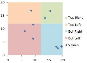
A popular graphical technique divides the plotting area of a chart into four quadrants, to facilitate such analyses as risk-reward. For example, one axis shows risk and the other shows reward; the quadrants divide risk and reward into low and high regions, and the quadrants show the combinations (low risk-high reward, low risk-low reward, etc.).

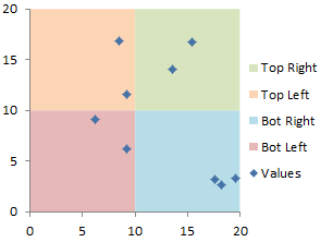
Chart with colored quadrant background

This technique is not difficult to follow in Excel. The plotted points are in an XY series, while the colored quadrants are formed by stacked area chart series.

First, The Data

All of the data needed to build a chart with colored quadrants is shown in the screen shot below. The individual values to be plotted are in the blue shaded range, B2:C11. The axis scales I want to use are in the green tinted range, B13:D15. The data needed for the area chart series is in the light orange range, B18:G25.

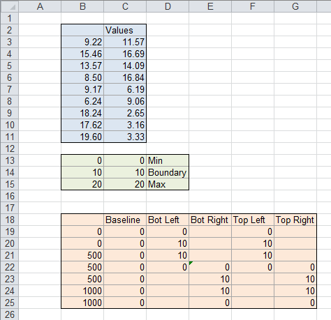
Data for chart with colored quadrant background

The orange (area chart) data range contains some formulas. The Baseline column is needed to ensure the same behavior in all versions of Excel (2000 through 2010). I want to scale the area chart horizontal scale from 0 to 1000 to provide enough resolution in the chart. Cells B19:B20 contain the value 0, and cells B24:B25 contain the value 1000. Cell B21 contains the formula

=(B14-B13)/(B15-B13)*1000

to scale the vertical boundary to the desired point along the horizontal scale, and cells B22 and B23 link back to B21.

Cells C19:C25 link to cell C13.

Cells D19, D22, E22, E25, F19, F22, G22, and G25 also link to cell C13. Cell D20 contains the formula

=C14-C13

and cells D21, E23, and E24 link to cell D20. Cell F20 contains the formula

=C15-C14

and cells F21, G23, and G24 link to cell F20.

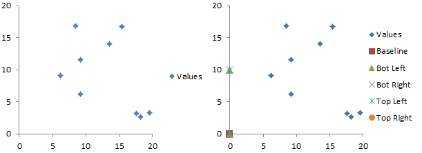
Select the blue range and insert an XY (Scatter) chart, markers only, to start the charting process (below left). Copy the orange range, select the chart, and use Paste Special to add the data to the chart as new series, with data in columns, and check the first column and first row boxes (below right). This may push all of the plotted values to the left of the chart, but I had set fixed maximum and minimum axis parameters.

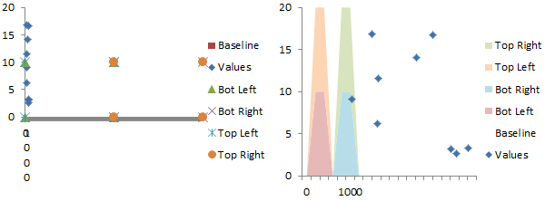
Creating chart with colored quadrant background

Change the Baseline series chart type to stacked area. This messes up the axes and scrunches the plotted values to the left of the chart (below left). Repeat for the Bottom Left, Bottom Right, Top Left, and Top Right series (below right). You may format the area series whenever you want. Keep in mind that Excel wants to use richly saturated colors, which will overwhelm the plotted points. I’ve used shades that are a couple steps lighter than the default fill colors. Also keep in mind that the Baseline series should be made transparent (no fill).

Creating chart with colored quadrant background

Format the Values series, and move it to the Secondary axis. This provides a secondary vertical axis (below left). On the Chart Tools > Layout tab, click on Axes, and select the default Secondary Horizontal Axis option, which gives us the top of the plotting rectangle (below right).

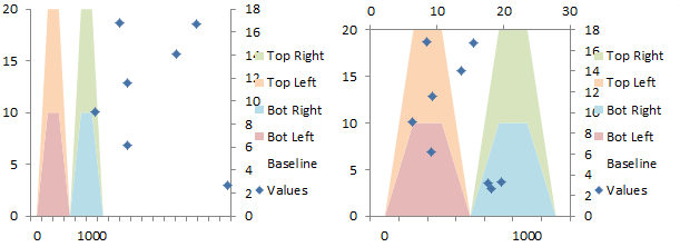
Creating chart with colored quadrant background

Format the left vertical axis, and under Horizontal Axis Crosses, select Maximum Axis Value (below left). Then format the right vertical axis, and under Horizontal Axis Crosses, select Automatic (below right).

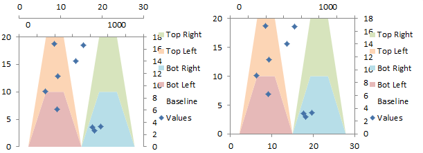
Creating chart with colored quadrant background

Select the right vertical axis, and press Delete (below left). Format the top horizontal axis: under Axis Type, select Date Axis; for Axis Labels, select None; for Line Color, select No Line (below right); and under Position Axis, choose On Tick Marks.

Creating chart with colored quadrant background

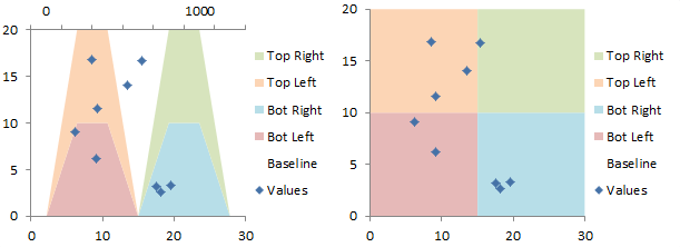
Resize the plot area if necessary (you’ll have to select Plot Area from the selection dropdown at the top left of the Chart Tools > Layout or Format tabs) and adjust any other formatting. Remove the unneeded Baseline legend entry by clicking once to select the legend and again on the “Baseline” label to select the legend entry, then press Delete. Don’t forget that Excel wants to use richly saturated colors for the area fills, which will overwhelm your value markers. Used colors that are a couple shades lighter than the defaults. Your chart is finished.

Chart with colored quadrant background

You can change where the quadrant borders appear by changing the values in cells B14 and C14.

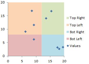
Chart with colored quadrant background

The chart adjusts as soon as you change these values.

Chart with colored quadrant background

Related Posts:

Posted: Wednesday, September 14th, 2011 under Combination Charts.
Comments: 61

Comments

Comment from Joe Mako
Time: Wednesday, September 14, 2011, 1:14 pm

Thanks for putting this together Jon,

I recreated this kind of view in Tableau, but instead of a static mid point, I have it based on the median value, along with a select-able legend for filtering the view:
http://public.tableausoftware.com/views/ColoredQuadrant/ColoredQuadrant

Comment from Jon Peltier
Time: Wednesday, September 14, 2011, 1:50 pm

Joe -

Good stuff. I’m jealous of the easy filtering. I could do it with checkboxes etc, but it always takes a couple minutes.

The cells that contain the border values could always contain a formula, so the borders could indicate median or any other calculated value. That’s easy in Excel, so I’m not jealous of that.

Comment from Leonid
Time: Wednesday, September 14, 2011, 6:04 pm

When dynamic nature of a colored background is not required the quick and simple way to achive this is to color in a desired way a contiguous range of cells with proportional rows and colomns count, copying them on a clipboard and formatting Plot Area as Fill->Picture or texture fill->Clipboard.

Comment from laguerriere
Time: Thursday, September 15, 2011, 4:40 am

Hello Jon

thank you again for a cool tutorial. I already know that I could use it for the pain-gain matrix for our consulting presentations. Need to figure out how to add 6 quandrants though and combine it with bubble charts.

I have only one problem: I did everything like you described but the Bot Left is not coloured… It’s white on the chart and pink on the legend. Very weird.

Maybe you could help to find out why? Here is the workbook
http://www.4shared.com/file/u9UYM3pU/PTS-chart-with-colored-quadran.html

Thank you in advance!

Pingback from Colors, Legends, and Labeling | Bootstrapping Life
Time: Thursday, September 15, 2011, 8:08 am

[...] colors and legends are not always a good method for creating a graph. The chart below from this post reminded me of this important point. The colors in the legend have no intuitive meaning and this is [...]

Comment from Eric
Time: Friday, September 16, 2011, 11:47 am

Jon,

I’ve been trying to automate this process (so that the user can provide data and Min/Boundary/Max values). I’ve got it so that everything works through the penultimate step (where you select Date Axis etc and the chart magically goes from being funky pyramids to the quadrants when you do this manually). I’ve checked the settings after I use VBA to set the Date Axis, Axis Labels to None, and Line Color to none and it seems to be the same as when I do the whole process manually and the chart changes to quadrants. Any idea why VBA doesn’t make the magic change from pyramids to quadrants?

I am working on an isolated LAN (w/Excel 2007) so I can’t give you the code, but I tried it at home with Excel 2010 last night and got the same incomplete results. Again, everything looks like the blog post through the very last step.

Any ideas?

Eric

Comment from Eric
Time: Friday, September 16, 2011, 2:02 pm

Jon,

I think that the problem may be associated with the change to Date Axis for axis type. I did this by:

ActiveChart.Axes(xlCategory).CategoryType = xlTimeScale

When this is done, the option button goes to the Date Axis option, but the change in the Format Axis box doesn’t show the Axis Options that you get when you do the change manually (i.e., Min, Max, Major/Minor units, Base unit, etc).

When I recorded the macro for this step, the only thing that was recorded was the above VB step. Did I miss something?

Thanks,

Eric

Comment from Eric
Time: Friday, September 16, 2011, 6:58 pm

@laguerriere

I am having the same problem with Bottom Left in my macro version of this blog entry. Let me know if you figure it out.

Thanks,

Eric

Comment from DaleW
Time: Saturday, September 17, 2011, 10:28 am

Jon,

Using Excel 2003, I got the same result as laguerriere and Eric: the Bot Left quadrant was the background color of the plot area (white by default).

Obviously, this was where I changed the plot area color and declared success. You might have a more elegant solution.

Thank you for this latest combo chart tutorial. (I can understand why Numbers on the iPad doesn’t even try to support combo charts imported from Excel.)

Comment from Jon Peltier
Time: Saturday, September 17, 2011, 3:29 pm

Okay, to all of you who had a blank bottom left quadrant, I apologize. I did this tutorial with that bastard child of Microsoft, Excel 2007.

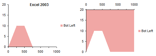
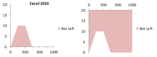
In Excel 2003 and 2010, an area chart series fills between the category axis and the data. If the category axis is at the bottom, it fills below the data. If the axis is at the top, it fills above the data. So if you’re paying attention, the area under the bottom left series is blank in the last three charts with trapezoids, and the area above the upper trapezoids is no longer blank, but has the fill color of the bottom left series.

Excel 2003: Area chart fills between axis and data.

Excel 2010: Area chart fills between axis and data.

Excel 2007: Area chart fills below data.

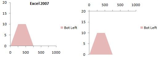
The other area series look the same in all versions, because these stack on top of the first series, that is, on top of the data of the first series.

I’ve corrected this protocol by inserting a dummy transparent series with values equal to the minimum of the vertical axis. This series will always reach to the bottom of the chart, as in the >500 half of the charts shown in this comment.

Comment from laguerriere
Time: Monday, September 19, 2011, 5:10 am

Thank you Jon, it works now!

Comment from James
Time: Monday, September 19, 2011, 1:43 pm

Hi Jon,

Thanks for your renewed colored quadrant method.
Building on it, I am trying to replace markers with oval shapes to simulate a bubble chart, but I am now facing the obstacle of the new series index.
As I paste a new series collection, is there a way to “force” the index number in order to attach shapes in a consistent way ?

Thanks a lot for your insight.

Comment from Jon Peltier
Time: Monday, September 19, 2011, 3:43 pm

James -

The last series you add should be

ActiveChart.SeriesCollection(ActiveChart.SeriesCollection.Count)

You can also give each series a unique name and call it using

ActiveChart.SeriesCollection(“UniqueSeriesName”)

Comment from Jon Peltier
Time: Monday, September 19, 2011, 4:15 pm

Eric :

Here’s what the Excel 2010 recorder gave me:

Sub Macro3()
    ActiveChart.Axes(xlCategory).Select
    ActiveChart.Axes(xlCategory).CategoryType = xlTimeScale
    ActiveChart.Axes(xlCategory).MaximumScale = 40
    ActiveChart.Axes(xlCategory).MajorUnit = 1
    ActiveChart.Axes(xlCategory).MajorUnit = 10
    ActiveChart.Axes(xlCategory).BaseUnit = xlDays
    ActiveChart.Axes(xlCategory).AxisBetweenCategories = False
End Sub

which can be rewritten:

Sub Macro3()
  With ActiveChart.Axes(xlCategory)
    .CategoryType = xlTimeScale
    .MaximumScale = 40
    .MajorUnit = 10
    .BaseUnit = xlDays
    .AxisBetweenCategories = False
  End With
End Sub

Comment from James
Time: Tuesday, September 20, 2011, 1:50 am

Hi Jon,

Thanks for your answer.
You are right … and I already gave a unique name to each of the four series.

My problem is that I can loop thru Series Index integers with ActiveChart.SeriesCollection.Count, but I do not know how to loop thru the Array made of the four UniqueSeriesNames …

Thanks again for your kind assistance.

Comment from James007
Time: Tuesday, September 20, 2011, 10:30 am

Hi Jon,

To solve my problem, I have written some not very elegant code …
Within the SeriesCollection.Count loop, I have inserted another loop on each item of the reference array, in order to have each item tested against each series collection unique name … which, in turn, allows to assign the right oval shape to each series.

Thanks again for your very helpful blog.

Comment from Eric
Time: Tuesday, September 20, 2011, 11:47 am

Jon,

Thanks, that helped a lot. However, I still have a problem if I try to set the quadrant data series through code and not by referencing a range on a worksheet.

The problem seems to me to be that I can’t set some of the values of the quadrant series data to be empty or null. When you paste in values to the chart using Paste Special, you have empty values for some of the cells in Baseline, Bottom Left, etc.

For specifying the values of the quadrant’s series in code, those “blank” values come up as either 0′s or as #N/A (when I use the keyword Empty) and you get the pyramids again. If I use a helper worksheet (which remains hidden to the user) or hide the quadrant series from the user the code version will work and I get the ultimate product. But my goal is to not have the hidden helper sheet or ranges.

For example, here’s the part of the code that puts in the series for the Bottom Left:

‘Add Bottom Left Series
Set ns = ch.SeriesCollection.NewSeries
With ns
.XValues = Array(0, _
0, _
Resolution * (BoundaryX – MinX) / (MaxX – MinX), _
Resolution * (BoundaryX – MinX) / (MaxX – MinX), _
Resolution * (BoundaryX – MinX) / (MaxX – MinX), _
Resolution, _
Resolution)
.Values = Array(0, _
BoundaryY, _
BoundaryY, _
0, _
Empty, _
Empty, _
Empty)
.Name = “Bottom Left”
.ChartType = xlAreaStacked
End With

You can put in 0′s for the Empty… same result = pyramids.

Any ideas on how to set the series values so that the right points get ignored?

Thanks for your help, and thanks for this great blog,

Eric

Comment from Jon Peltier
Time: Tuesday, September 20, 2011, 1:33 pm

Eric -

You should be able to use zeros instead of “empty”.

You could use either of these to enter an array into the chart:

ActiveChart.SeriesCollection(1).Values = Array(1, 3, 42.5, 2, 0, 0)
ActiveChart.SeriesCollection(1).Values = “={1, 3, 42.5, 2, 0, 0}”

As long as you have defined the category type of the correct category axis as xlTimeScale, you should get boxes.

Pingback from Campaign Intensity, Negativity, and Using Color to Represent Quantitative Variables
Time: Tuesday, September 20, 2011, 4:00 pm

[...] posted a similar graph of faked data in a recent blog in which I discussed Jon Peltier’s mapping of non-intuitive colors to qualitative variables. Jon was kind enough to provide thoughtful feedback on my graph and we [...]

Comment from Eric
Time: Tuesday, September 20, 2011, 4:52 pm

Jon,

Nope. If you specify the values in code (as either 0 or Empty) that are empty in the orange block, you get pyramids (trapezoids, actually, I guess). If you specify the values as a range, you get quadrants.

The interesting thing remains the format options for the horizontal axis. I put a break on the code after entering the series values and moving the point values (the blue box data) to the secondary axis. If you specify the values for the quadrant data in code and then try to set the horizontal axis to a date axis, the format box will not change and so not give you options to set min/max etc values for the axis. If you specify a range and try this, it will.

So I guess that I’ll have to maintain the quadrant data either on a helper sheet or somewhere on the data sheet. I was trying to avoid that.

Thanks anyway,

Eric

Comment from Jon Peltier
Time: Tuesday, September 20, 2011, 10:17 pm

Eric -

I ran this in Excel 2007 SP2 (make sure you have SP2 installed), and it made a nice 4-quad chart background.

Sub MakeChart()
  Dim cht As Chart
  Dim srs As Series

  Set cht = ActiveSheet.ChartObjects.Add(25, 25, 350, 300).Chart
  cht.ChartArea.ClearContents

  Set srs = cht.SeriesCollection.NewSeries
  With srs
    .Values = Array(0, 50, 50, 0, 0, 0, 0)
    .XValues = Array(0, 0, 500, 500, 500, 1000, 1000)
    .Name = "Bottom Left"
    .ChartType = xlAreaStacked
  End With

  Set srs = cht.SeriesCollection.NewSeries
  With srs
    .Values = Array(0, 0, 0, 0, 50, 50, 0)
    .XValues = Array(0, 0, 500, 500, 500, 1000, 1000)
    .Name = "Bottom Right"
    .ChartType = xlAreaStacked
  End With

  Set srs = cht.SeriesCollection.NewSeries
  With srs
    .Values = Array(0, 50, 50, 0, 0, 0, 0)
    .XValues = Array(0, 0, 500, 500, 500, 1000, 1000)
    .Name = "Top Left"
    .ChartType = xlAreaStacked
  End With

  Set srs = cht.SeriesCollection.NewSeries
  With srs
    .Values = Array(0, 0, 0, 0, 50, 50, 0)
    .XValues = Array(0, 0, 500, 500, 500, 1000, 1000)
    .Name = "Top Right"
    .ChartType = xlAreaStacked
  End With

  With cht.Axes(xlCategory)
    .CategoryType = xlTimeScale
    .MinimumScale = 0
    .MaximumScale = 1000
    .MajorUnit = 200
    .MajorUnitScale = xlDays
    .BaseUnit = xlDays
    .AxisBetweenCategories = False
  End With

  With cht.Axes(xlValue)
    .MinimumScale = 0
    .MaximumScale = 100
    .MajorUnit = 20
  End With

End Sub

Comment from Jon Peltier
Time: Tuesday, September 20, 2011, 10:32 pm

Eric -

This one includes the XY series, and does the axis stuff.

Sub MakeChart2()
  Dim cht As Chart
  Dim srs As Series

  Set cht = ActiveSheet.ChartObjects.Add(25, 25, 350, 300).Chart
  cht.ChartArea.ClearContents

  Set srs = cht.SeriesCollection.NewSeries
  With srs
    .Values = Array(0, 0, 0, 0, 0, 0, 0)
    .XValues = Array(0, 0, 500, 500, 500, 1000, 1000)
    .Name = "Baseline"
    .ChartType = xlAreaStacked
  End With

  Set srs = cht.SeriesCollection.NewSeries
  With srs
    .Values = Array(0, 50, 50, 0, 0, 0, 0)
    .XValues = Array(0, 0, 500, 500, 500, 1000, 1000)
    .Name = "Bottom Left"
    .ChartType = xlAreaStacked
  End With

  Set srs = cht.SeriesCollection.NewSeries
  With srs
    .Values = Array(0, 0, 0, 0, 50, 50, 0)
    .XValues = Array(0, 0, 500, 500, 500, 1000, 1000)
    .Name = "Bottom Right"
    .ChartType = xlAreaStacked
  End With

  Set srs = cht.SeriesCollection.NewSeries
  With srs
    .Values = Array(0, 50, 50, 0, 0, 0, 0)
    .XValues = Array(0, 0, 500, 500, 500, 1000, 1000)
    .Name = "Top Left"
    .ChartType = xlAreaStacked
  End With

  Set srs = cht.SeriesCollection.NewSeries
  With srs
    .Values = Array(0, 0, 0, 0, 50, 50, 0)
    .XValues = Array(0, 0, 500, 500, 500, 1000, 1000)
    .Name = "Top Right"
    .ChartType = xlAreaStacked
  End With

  Set srs = cht.SeriesCollection.NewSeries
  With srs
    .Values = Array(25, 75, 40, 80, 65, 30)
    .XValues = Array(35, 20, 60, 45, 85, 75)
    .Name = "XY Data"
    .ChartType = xlXYScatter
    .AxisGroup = xlSecondary
  End With

  cht.HasAxis(xlCategory, xlSecondary) = True
  cht.HasAxis(xlValue, xlSecondary) = True

  With cht.Axes(xlValue, xlSecondary)
    .Crosses = xlAxisCrossesAutomatic
    .MinimumScale = 0
    .MaximumScale = 100
    .MajorUnit = 20
  End With

  With cht.Axes(xlCategory, xlPrimary)
    .CategoryType = xlTimeScale
    .MinimumScale = 0
    .MaximumScale = 1000
    .MajorUnit = 200
    .MajorUnitScale = xlDays
    .BaseUnit = xlDays
    .AxisBetweenCategories = False
    .TickLabelPosition = xlTickLabelPositionNone
    .Border.LineStyle = xlNone
  End With

  With cht.Axes(xlValue, xlPrimary)
    .Crosses = xlAxisCrossesMaximum
    .MinimumScale = 0
    .MaximumScale = 100
    .MajorUnit = 20
  End With

  cht.HasAxis(xlValue, xlSecondary) = False

End Sub

Comment from Eric
Time: Wednesday, September 21, 2011, 10:05 am

Jon,

Just tried the second version on a box with Excel 2007 with SP2 installed. It errors out in the

With cht.Axes(xlCategory, xlPrimary)

section on the

.MajorUnitScale = xlDays

statement with a

Run time error ‘-2147467256 (80004005)’:
Invalid Parameter

Again, when I check the format box of the Horizontal Axis (primary, i.e., top one) I do not see the options for setting min/max/major unit / minor unit values.

So what setting am I missing somewhere in the bowels of Excel? That’s got to be the answer, right?

Thanks for helping,

Eric

Comment from Jon Peltier
Time: Wednesday, September 21, 2011, 10:38 am

Eric -

Yeah, now that I test in 2010, I’m getting that same error. I’m looking into it.

Comment from Jon Peltier
Time: Wednesday, September 21, 2011, 11:20 am

Eric -

No joy. I’ve tried a number of things. I even created the series using dummy worksheet ranges. As soon as the data for any of the series is entered as (or changed to) an array, the date axis breaks. The date axis option is selected, but the scaling parameters are those of a category axis.

This is the first charting thing I’ve encountered that works worse in Excel 2010 than in 2007.

Comment from Alison
Time: Thursday, September 22, 2011, 6:48 pm

Genius! Thanks so much!

Comment from Eric
Time: Thursday, September 22, 2011, 6:51 pm

Thanks for trying, Jon. I am going with the Helper sheet option… Ah well.

Cheers,

Eric

Pingback from “Quadrant” for Data Visualization Platforms « Data Visualization
Time: Monday, September 26, 2011, 10:13 pm

[...] am going to update using method suggested by Jon Peltier: http://peltiertech.com/WordPress/excel-chart-with-colored-quadrant-background/ – Thank you Jon! I hope I will have time before end of 2011 for [...]

Comment from Anonymous
Time: Thursday, November 10, 2011, 2:04 pm

What version of Excel are you using for this? I use Excel 2002 (10.6834.6830) SP3 at work and don’t have the option to upgrade.

Alot of the things you refer to don’t seem to exist in my version of Excel like “Chart Tools > Layout tab” and “stacked area” chart as in “Change the Baseline series chart type to stacked area.” I can’t find these things.

I wish you (and all other experts who write tutorials) would explain everything in the greatest detail possible or include foot notes that would explain things in details.

Pingback from Excel 2003 Rectangle de couleur dans graph type bulle
Time: Monday, November 21, 2011, 12:11 pm

[...] [...]

Comment from chatupon
Time: Tuesday, November 29, 2011, 4:39 am

Your makechart so cool!
But can you show how to show datalabel on mark? (it should show data of third column)

Comment from 3G
Time: Wednesday, November 30, 2011, 2:18 pm

Hey Jon-
Love the technique! I am going to use this as a risk quad chart, and, would like to be able to add data labels (i.e. a “risk Number”) to the 10 points I’m going to plot. How can I add this info?

Thanks for all of the awesome posts!
3G

Comment from Jon Peltier
Time: Wednesday, November 30, 2011, 5:12 pm

GGG -

To label points, check out Rob Bovey’s Chart Labeler, at http://appspro.com.

Comment from CW
Time: Tuesday, February 7, 2012, 3:09 pm

Hi,

This is cool stuff. But what if I only want the green and blue areas shaded – and shaded the same color even. So I basically want the graph divided into 2/3 and 1/3 the last 1/3 is one color – essentially I am drawing attention to the part of a graph that is projection. How do I adapt the above formula?

Thanks!
Cecilia

Comment from Jon Peltier
Time: Tuesday, February 7, 2012, 10:53 pm

CW –

The last two charts in the article show how you can change the dividing parameters in B14:C14 to move the intersection of the colored regions. In your case say you want to shade only the last 1/4 of the chart. Change the value in B14 to 15 (which is 3/4 of 20). Then since you don’t want to shade the left part of the chart, you can delete the Bot Left and Top Left series. Also, since you only need one color in the right part of the chart, delete the Top Right series. To make the remaining area reach the top of the chart, change C14 to 20.

Comment from Mustafa
Time: Thursday, February 9, 2012, 5:06 pm

Hi Jon, amazing stuff! Works perfectly and nice brief explanation of the steps to go through!

I only have 1 question: is there a way to include the min-max values of the axes in a cell? Also right now I’m using percentages 0-100% for both my axes. Min quadrant border is set to 0 and max set to 1. Setting the boundary for the quadrants at for example 0,65 works perfectly, but gets messed up only for the HORIZONTAL axis when I change the minimum and maximum value. Any idea on how to cope with this?

Thanks in advance!

Comment from Jon Peltier
Time: Thursday, February 9, 2012, 6:02 pm

Mustafa -

The values being plotted are on the secondary axis, with whatever X and Y axis scales make sense.

The area series that provide the shaded quadrants are on the primary axis.

The primary X axis is date scale, with min=0 and max=1000, and these never change. The cut off between left and right quadrants is scaled between 0 and 1000 based on the min and max of the primary X axis and the value where you want the quadrants to meet. For example, if the plotted points have an axis that goes from 0% to 100% and you want the quadrants to meet at 65%, the formulas should make this transition occur at 650 on the primary X axis.

The primary Y axis is the only Y axis, since the secondary one was deleted. This ensures that the Y values of the plotted points and of the quadrants are synchronized to one scale.

Comment from Mustafa
Time: Friday, February 10, 2012, 2:51 am

Thanks for your quickly reply Jon! I got it sorted out based on a simple formula like you described:
=((quadrant border-min. axis value)/((max. axis value-min. axis value)/100))/100

Only downside is that I have to rescale the actual axis of the graph manually via the format axis menu, but I think I can live with that.

Mustafa

Comment from CW
Time: Tuesday, February 14, 2012, 11:02 am

“Change the Baseline series chart type to stacked area.”

This step makes my excel crash every time. Anyway around it?

Comment from Jon Peltier
Time: Tuesday, February 14, 2012, 1:37 pm

CW -

That’s strange. What versions of Excel and Windows are you using? Can you change one of the other series? Can you make a stacked area chart to begin with?

Comment from CW
Time: Tuesday, February 14, 2012, 1:48 pm

Yeah well eventually it will do it however it loses the option for the “default” axis on the primary and/or secondary axis and there is no way to change the axis except for in date format.

Comment from Kim
Time: Tuesday, February 21, 2012, 2:02 am

Hi Jon,
Is it possible to divide the chart into 25 quadrants? Thanks.

Comment from Kim
Time: Tuesday, February 21, 2012, 4:47 am

Hi Jon,
After deleting the right vertical axis, can you reiterate the steps to be performed to form the 4 quadrant? It seems so hard to convert the trapezoids into squares & quadrant. HELP please. Thanks.

Comment from Jon Peltier
Time: Tuesday, February 21, 2012, 10:41 am

Kim -

It’s possible to divide the background into more than a two-by-two pattern. This is what the data and resulting chart look like for a 5×5 background. The formulas would work the same as in this example.

After removing the right hand axis, you have stacked up trapezoids. To convert them to rectangles:

Format the top horizontal axis: under Axis Type, select Date Axis; for Axis Labels, select None; for Line Color, select No Line (below right); and under Position Axis, choose On Tick Marks.

Comment from Kim
Time: Thursday, February 23, 2012, 12:15 am

Thanks Jon.

However, i’m still having a hard time converting the trapezoid to rectangle. I already followed these steps:

Format the top horizontal axis: under Axis Type, select Date Axis; for Axis Labels, select None; for Line Color, select No Line (below right); and under Position Axis, choose On Tick Marks.

Hope I can send the file I’m working now. Thanks.

Comment from Kim
Time: Thursday, February 23, 2012, 3:56 am

I still can’t achieve the rectangle form. I must be missing something because after formatting the top horizontal axis, the shape is still trapezoid (only the top horizontal axis was removed).

Hope you can help me on this. Thanks.

Pingback from Excel 2010 Affichage zones sombres et claires sur un graphique pour imager nuits et jours
Time: Thursday, February 23, 2012, 8:23 am

[...] [...]

Comment from Jon Peltier
Time: Thursday, February 23, 2012, 9:23 am

Kim -

You didn’t include an email address, so I can’t send you a link for your file.

Comment from Kim
Time: Tuesday, February 28, 2012, 1:14 am

My email address is kim.anderson2726@yahoo.com Hope you can help me on this, please. I badly need to know how to construct a 5×5 quadrant for my project.

Thanks Jon.

Comment from Kim
Time: Thursday, March 1, 2012, 5:21 am

Hi Jon,
Hope you can help me. Thanks.

Kim

Comment from Al Pat
Time: Tuesday, March 13, 2012, 9:19 am

Hi Jon,
I am working on a project that needs 3 x 3 x 3 quadrant chart, I tried everyting you have shown above and was able to create 4 x 4 but am not sure how the formulas will work for 3x3x3 quadrant. My boundries are 3 and 6 on scale of 0 to 9 on both axes. Can you please help me?

Comment from Jon Peltier
Time: Wednesday, March 14, 2012, 8:27 am

Al -

If you can do 2×2 and 4×4, the 3×3 should be an easy adjustment.

Comment from Kim
Time: Tuesday, March 20, 2012, 4:20 am

Hi Jon,
Hope you can still help me in achieveing the final chart. I’m stucked up in trapezoid figure and can’t make it appear like quadrants. Hope I can send you my file so can see where I’m coming from?

Thanks.
Kim

Comment from Dom
Time: Thursday, April 12, 2012, 11:49 am

Jon, you’re a genious!
However, more explanatory would have been an example not crossing at zero, with different values for the horizontal and vertical axis and no crossing point of (10,10).
In my chart the min/max values are dynamic, as well as the crossing of the axis. However, as example x ranges from -6% to +2%, y ranges from 0% to 12%, crossing is at (-1%, 5.5%) and thus defines 4 quadrants. I’ll keep on guessing, at least I know now that its possible. Thanks, Dom.

Comment from Fred
Time: Wednesday, May 2, 2012, 3:16 am

Hi Jon,

I hope you are still following this thread.

I am desperately trying to apply this to a chart having to display severalseries as bubble chart, is it only possible? It would exactly match my needs.

I am building the chart in VBA, but I get plenty of errors. Is it compatible?

Many thanks already for your help,
Fred.

Comment from Jon Peltier
Time: Wednesday, May 2, 2012, 6:37 am

Fred -

You don’t mention what the error descriptions are, so it’s hard to comment specifically.

Bubble charts cannot be combined with other chart types. Since you’re using VBA already, you can use the approach here with an XY chart, use circles as your markers, and change the circle size based on a third column of data (much like bubble charts use a third column to control bubble size).

Comment from Cam
Time: Friday, May 4, 2012, 10:43 am

Hi Jon,

I’m experiencing something similar with the converting to quadrants. I change the axis to “Date” and it just spits out “The entry is invalid for the data used by this chart. Please enter a value that falls within the min and max data values used by this chart”

Any help would be great!

Thanks!

Comment from Dom
Time: Wednesday, May 16, 2012, 5:58 am

Dear Jon

with some VBA-Chart adjustments those quadrants can be made dynamic depending on the scatter plot values. Increments can be calculated in order to define Interval size and keep (0,0) in axis labelling, Min and Max values should be rounded (floor, ceiling). It’s very important to define the Secondary Vertical Axis crossing as C13.
Slight transparency of quadrant colors and gridlines (Primary Horizontal and Secondary Vertical Axis) get visible (for those whh like gridlines).
Here’s my code:

Sub ChartAdjustments()
ActiveSheet.ChartObjects(“chartName”).Activate
‘Define crossing of Secondary Vertival Axis
ActiveChart.SetElement (msoElementSecondaryValueAxisShow)
ActiveChart.Axes(xlValue, xlSecondary).Select
ActiveChart.Axes(xlValue, xlSecondary).CrossesAt = Range(“SVcross”).Value ‘=C13
ActiveChart.SetElement (msoElementSecondaryValueAxisNone)
‘Define Min, Max and Increment of Primary Vertical Axis
ActiveChart.Axes(xlValue).Select
ActiveChart.Axes(xlValue).MinimumScale = Range(“PVmin”).Value ‘=min(C3:C11)
ActiveChart.Axes(xlValue).MaximumScale = Range(“PVmax”).Value
ActiveChart.Axes(xlValue).MajorUnit = Range(“PVinc”).Value
‘Define Min, Max and Increment of Secondary Horizontal Axis
ActiveChart.Axes(xlCategory, xlSecondary).Select
ActiveChart.Axes(xlCategory, xlSecondary).MinimumScale = Range(“SHmin”).Value ‘=min(B3:B11)
ActiveChart.Axes(xlCategory, xlSecondary).MaximumScale = Range(“SHmax”).Value
ActiveChart.Axes(xlCategory, xlSecondary).MajorUnit = Range(“SHinc”).Value

‘B13 = min(B3:B11) ‘C13 = min(C3:C11)
‘B14, C14: dynamic of Range(“B3:B11″), (“C3:C11″)
‘B15 = max(B3:B11) ‘C15 = max(C3:C11)
End Sub

Best regards and thanks for your great work!
Dom

Comment from Jon Peltier
Time: Wednesday, May 16, 2012, 10:05 am

Dom -

You can do all kinds of things, limited only by (a) your imagination and (b) legibility of the graph. I recently built a chart that had dynamically sized quadrants and dynamically scaled axes, based on the scatter plot data. The client was thrilled.

Comment from Fred
Time: Wednesday, May 16, 2012, 11:04 am

@Dom

How do you set the Transaprency property of the series representing the quadrant colors?

I’m running MS Excel 2003 SP3, and I don’t see this property for the series or series.fill

Thanks,
Fred.

Comment from Jon Peltier
Time: Wednesday, May 16, 2012, 3:23 pm

Fred -

Transparency was introduced to graphical objects in Excel 2007.

Write a comment

I welcome comments from my readers. If you have an opinion on this post, if you have a question or if there is anything to add, I want to hear from you. Whether you agree or disagree, please join the discussion.

If you want to include an image in your comment, post it on your own site or on one of the many free image sharing sites, and include a link in your comment. I'll download your image and insert the necessary html to display the image inline.

Read the PTS Blog Comment Policy.