Excel Column Chart with Horizontal Line Segments.

This page shows a different way to indicate benchmark or target numbers on a column chart. The values of interest are shown by columns, while the benchmark or target level is indicated by a horizontal line above each category.

Start with data arranged like this, with category labels, benchmark data, and actual performance:

Create a standard clustered column chart.

Right click on the Benchmark series, choose Chart Type from the pop-up menu, and choose the XY Scatter type with markers and no lines.

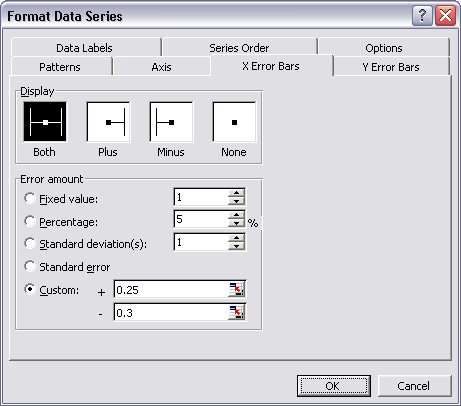
Add X error bars to the Benchmark series. You can enter a number in the Fixed Value box, but to me this appeared asymmetrical, so I entered unequal negative and positive values in the Custom boxes. For more on Error Bars, see Error Bars in Microsoft Excel Charts.

Double click on the Benchmark series, and on the Patterns tab, select None for Markers. Double click on the Benchmark error bars, and on the patterns tab, select an appropriate color and line thickness (in this example, a medium-weight blue line), and click on the Marker style without the perpendicular end caps.

There's an annoying divot in the top of the horizontal line formed by the error bars if you use no marker. A small (size 2) blue square fills in the divot nicely.

Add another series to serve as a legend entry for the Benchmark error bars. I copied A1:B3 from the worksheet, selected the chart, used Paste Special from the Edit menu, and chose the New Series option.

Format the dummy Benchmark series to match the error bars (i.e., a thick blue line).

Hide the dummy Benchmark series. I did this by changing the X value data range from B2:B3 to D2:D3, using Source Data on the Chart menu, on the Series tab. D2:D3 is blank, so it will not appear in the chart, but the series remains in the legend.

Remove the original "Benchmark" legend entry. Click once to select the legend, again on the label to select it, then press Delete. I've also moved the legend to the top of the chart.

Peltier Technical Services, Inc.

Excel Chart Add-Ins | Training | Charts and Tutorials | PTS Blog

Peltier Technical Services, Inc., Copyright © 2017. All rights reserved.
You may link to this article or portions of it on your site, but copying is prohibited without permission of Peltier Technical Services.

Microsoft Most Valuable Professional

My MVP Profile